ggplot2 and dplyr
Review
A quick review before we get into more complicated exercises:
#Load in your data
penguins <- read.csv("penguins.csv")

#Look at the column names and types of your data using str()
str(penguins)
## 'data.frame': 344 obs. of 8 variables:
## $ species : chr "Adelie" "Adelie" "Adelie" "Adelie" ...
## $ island : chr "Torgersen" "Torgersen" "Torgersen" "Torgersen" ...
## $ bill_length_mm : num 39.1 39.5 40.3 NA 36.7 39.3 38.9 39.2 34.1 42 ...
## $ bill_depth_mm : num 18.7 17.4 18 NA 19.3 20.6 17.8 19.6 18.1 20.2 ...
## $ flipper_length_mm: int 181 186 195 NA 193 190 181 195 193 190 ...
## $ body_mass_g : int 3750 3800 3250 NA 3450 3650 3625 4675 3475 4250 ...
## $ sex : chr "male" "female" "female" NA ...
## $ year : int 2007 2007 2007 2007 2007 2007 2007 2007 2007 2007 ...#Make a scatter plot of *body mass* and *bill depth*
ggplot(penguins, aes(x = body_mass_g, y = bill_depth_mm)) + geom_point()## Warning: Removed 2 rows containing missing values (geom_point).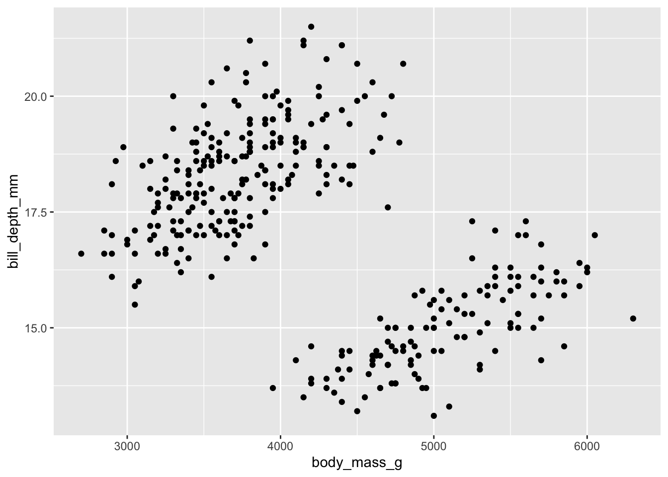
#Make a density plot of body mass with a fill color changing by sex and a transparency of 0.4
ggplot(penguins, aes(x = body_mass_g, fill = sex)) + geom_density(alpha = 0.4)
## Warning: Removed 2 rows containing non-finite values (stat_density).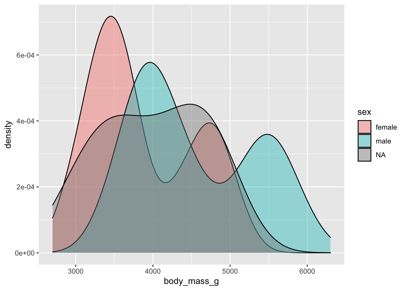
#Name the density plot above using ggtitle()
ggplot(penguins, aes(x = body_mass_g, fill = sex)) + geom_density(alpha = 0.4) + ggtitle("Body Mass by Sex")
## Warning: Removed 2 rows containing non-finite values (stat_density).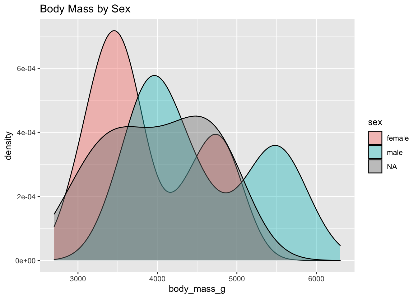
Practice Exercise
With a partner, let’s make a scatter plot and two density plots of two numeric variables; make one scatter plot looking at the correlation between the two, and then a density plot for each variable that you choose. Color based on a categorical variable.
# Use head() or str() to find the variables that are numeric
str(penguins)
## 'data.frame': 344 obs. of 8 variables:
## $ species : chr "Adelie" "Adelie" "Adelie" "Adelie" ...
## $ island : chr "Torgersen" "Torgersen" "Torgersen" "Torgersen" ...
## $ bill_length_mm : num 39.1 39.5 40.3 NA 36.7 39.3 38.9 39.2 34.1 42 ...
## $ bill_depth_mm : num 18.7 17.4 18 NA 19.3 20.6 17.8 19.6 18.1 20.2 ...
## $ flipper_length_mm: int 181 186 195 NA 193 190 181 195 193 190 ...
## $ body_mass_g : int 3750 3800 3250 NA 3450 3650 3625 4675 3475 4250 ...
## $ sex : chr "male" "female" "female" NA ...
## $ year : int 2007 2007 2007 2007 2007 2007 2007 2007 2007 2007 ...# Make a scatter plot of the two variables using geom_point()
# Add a color to separate the categorical variable
penguins %>%
ggplot(., aes(x = bill_length_mm, y = body_mass_g, color = island)) +
geom_point() +
# Add axis labels and a title to your plot
xlab("Bill Length (mm)") +
ylab("Body Mass (g)") +
ggtitle("Does a heavier penguin have a longer bill?")## Warning: Removed 2 rows containing missing values (geom_point).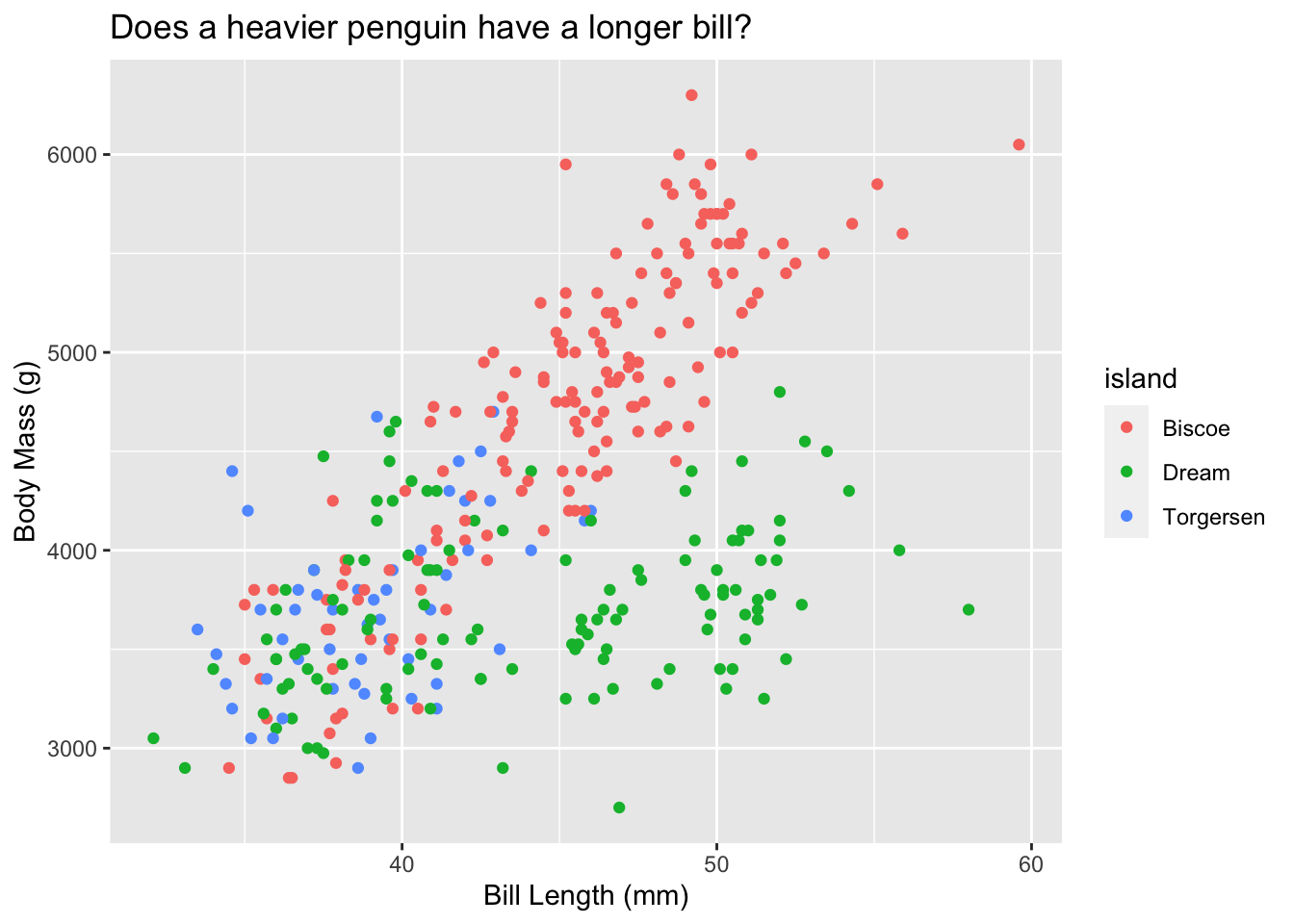
#Make a density plot using geom_density()
penguins %>%
  ggplot(., aes(x = bill_length_mm, color = island)) +
  geom_density() +
# Add axis labels and a title to your plot using ggtitle(), xlab(), and ylab()
  xlab("Bill Legnth (mm)") +
  ylab("Density") +
  ggtitle("Density distribution")
## Warning: Removed 2 rows containing non-finite values (stat_density).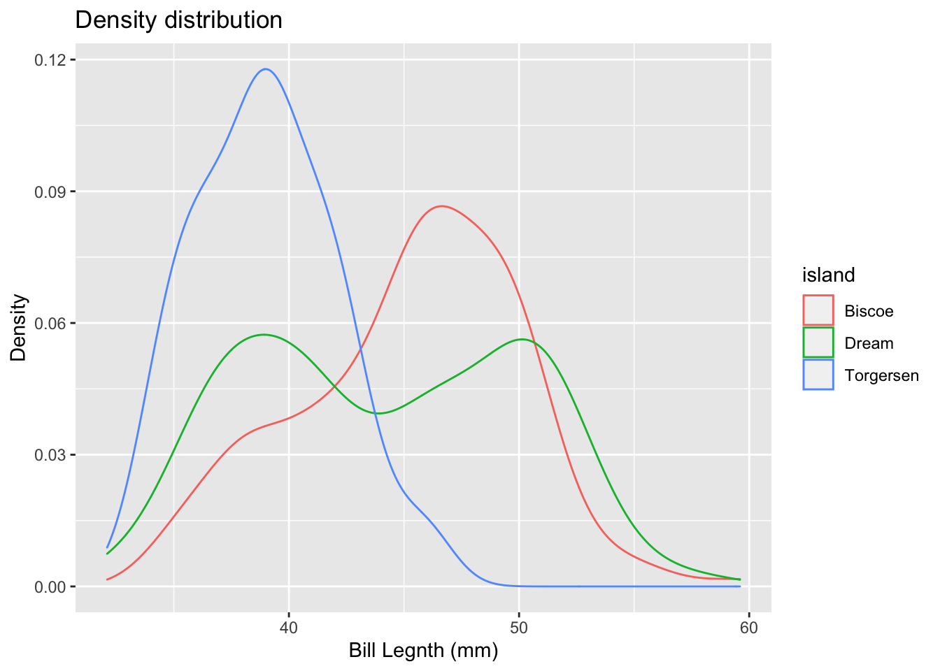
# Share with the class which variables you chose and what your plots looked likeUsing Dplyr to pipe into plotting
So far we’ve included into ggplot() the arguments for data and columns, but we can also use dplyr to pipe. In dplyr, the argument being used is often referred to as ‘.’, so using this can allow you to substitute based on your other pipeline arguments.
penguins %>%
  ggplot(data = .,aes(x = body_mass_g, color = species)) +
  geom_density(size = 2)
## Warning: Removed 2 rows containing non-finite values (stat_density).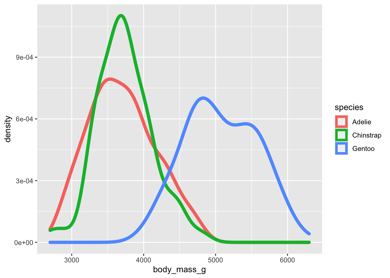
penguins %>%
  filter(species == "Adelie") %>%
  ggplot(data = .,aes(x = body_mass_g, color = species)) +
  geom_density(size = 2)
## Warning: Removed 1 rows containing non-finite values (stat_density).
Omitting NAs
We can also use the dplyr function na.omit() to remove the NAs in our dataset before plotting.
#Original graph
penguins %>%
  ggplot(., aes(x = body_mass_g, fill = sex)) +
  geom_density(alpha = 0.4) +
  ggtitle("Body Mass by Sex")
## Warning: Removed 2 rows containing non-finite values (stat_density).
#New graph
penguins %>%
  na.omit() %>%
  ggplot(., aes(body_mass_g, fill = sex)) +
  geom_density(alpha = 0.4) +
  ggtitle("Body Mass by Sex")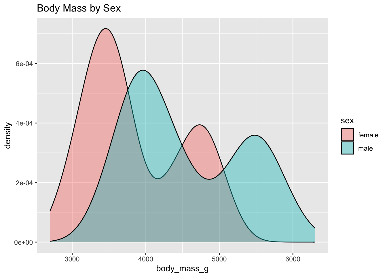
Practice
# Using piping, filter to only the female Adelie penguins and plot their bill length vs bill depth
#Color this plot by island
penguins %>%
  filter(species == "Adelie", sex == "female") %>%
  ggplot(., aes(x = bill_length_mm, y = bill_depth_mm, color = island)) +
  geom_point()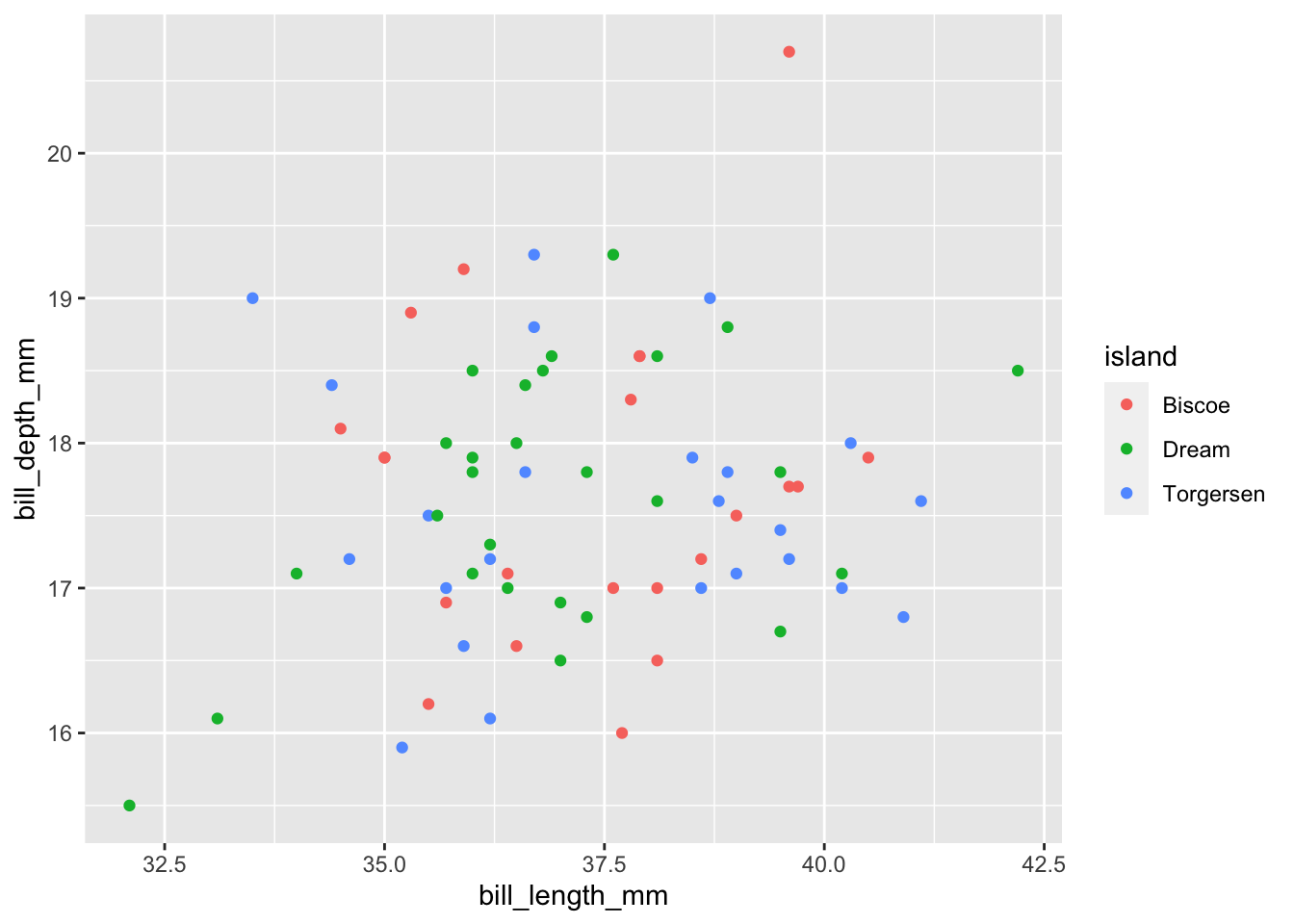
# Change the size to be 3 and the transparency of your points to 0.5
penguins %>%
  filter(species == "Adelie", sex == "female") %>%
  ggplot(., aes(x = bill_length_mm, y = bill_depth_mm, color = island)) +
  geom_point(size = 3, alpha = 0.5)
# Label your plot and include a title
penguins %>%
  filter(species == "Adelie", sex == "female") %>%
  ggplot(., aes(x = bill_length_mm, y = bill_depth_mm, color = island)) +
  geom_point(size = 3, alpha = 0.5) +
  xlab("Bill Length (mm)") +
  ylab("Bill Depth (mm)") +
  ggtitle("I ♥ Adelie Penguins")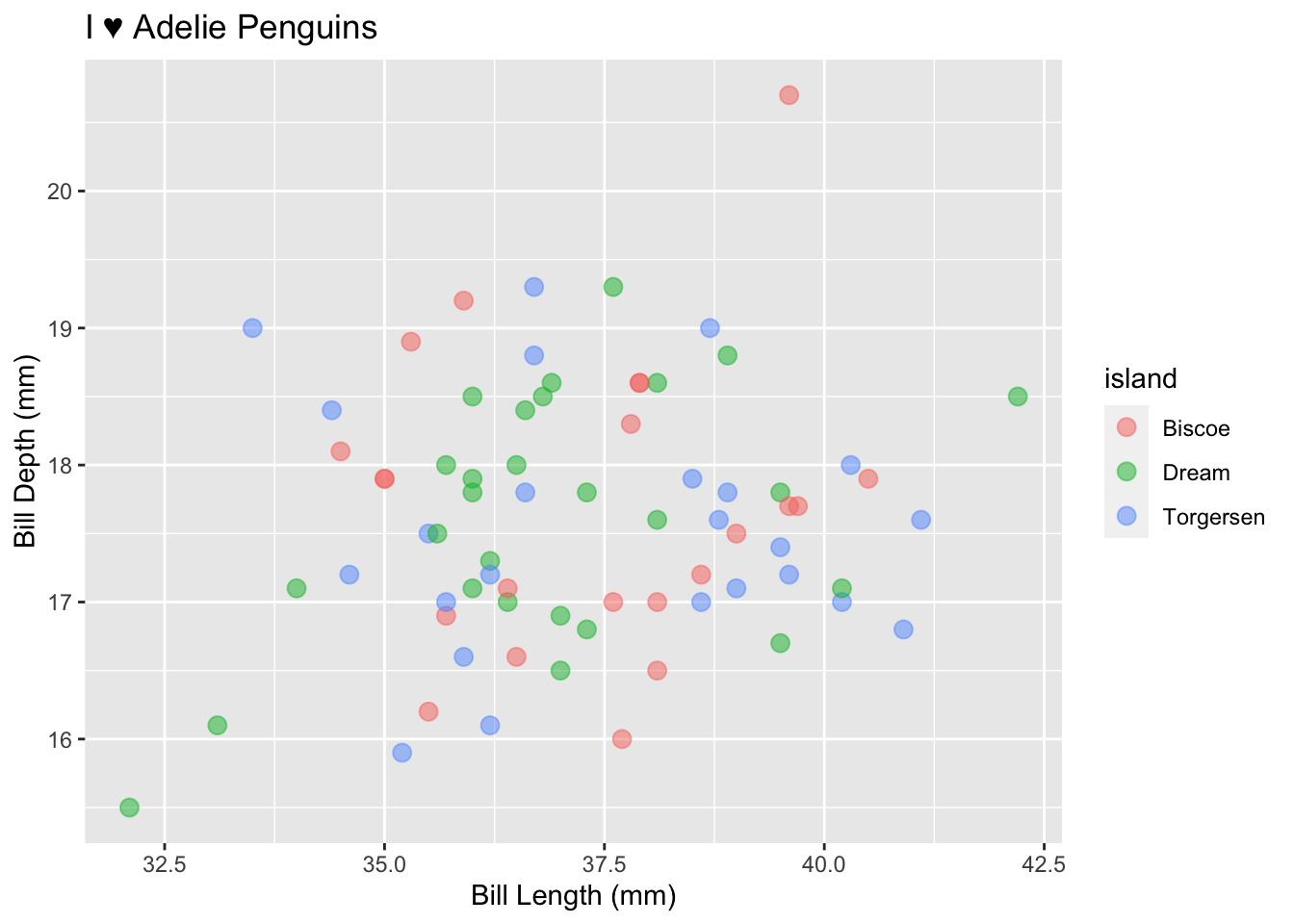
Bar Plots
We’ve mostly looked at numeric data; but what about using categorical data on our x or y axis? Bar plots are one way to look at this, and they have multiple functions for a bar-like graph. Here we’ll go through a few
Counts
#To count the number of individuals
penguins %>% ggplot(., aes(x = species)) + geom_bar()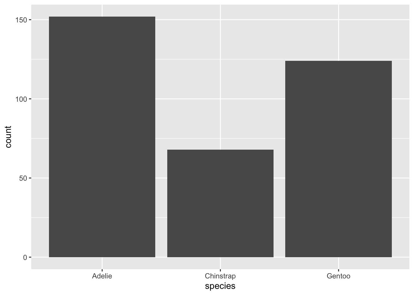
#Adding in color to separate by sex
penguins %>% ggplot(., aes(x = species, fill = sex)) + geom_bar()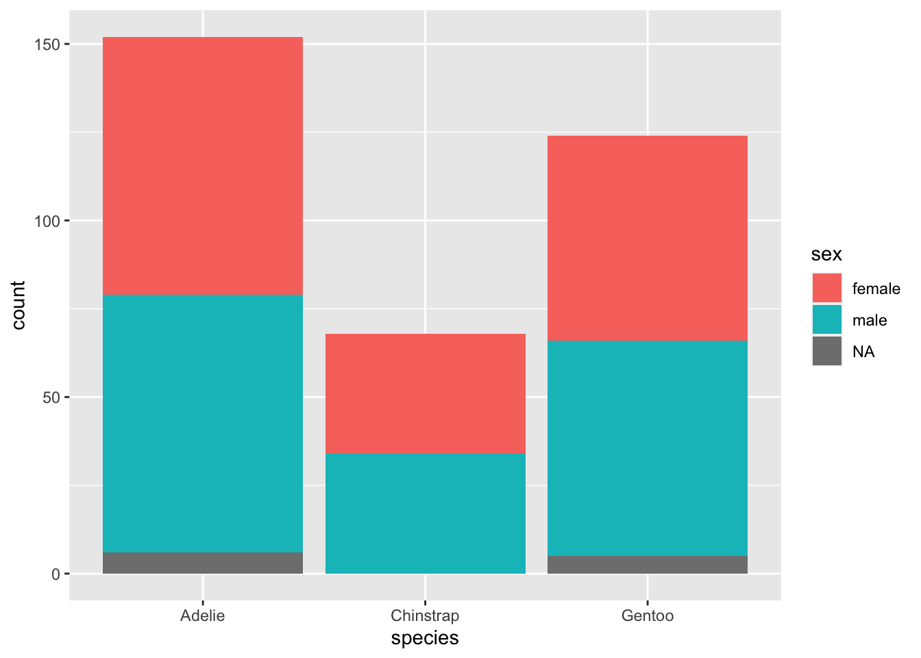
#Changing the position to
penguins %>% na.omit() %>% ggplot(., aes(x = species, fill = sex)) + geom_bar(position = "dodge")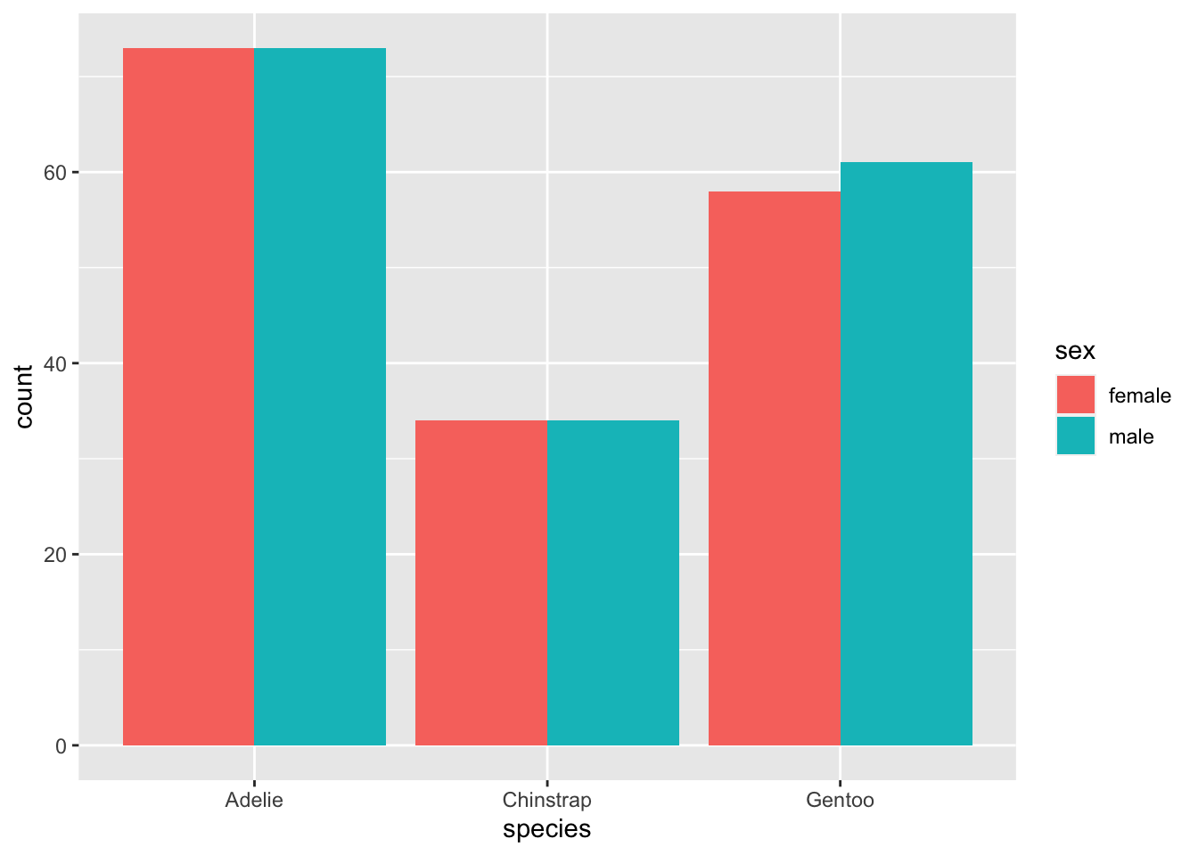
Values
Instead of the automatic counts that we get in geom_bar(), we can use geom_col() to produce columns that represent the measure of choice. Keep in mind that bar graphs of either type will start at 0, and so the scale might not be a good representation of differences. Since it is possible to change the y axis, keep in mind that you should almost NEVER do this on a bar plot because it looks misleading and enhances the differences in disproportionate ways. Other plots are better suited.
penguins %>% na.omit() %>% group_by(species) %>% summarize(mean_bill = mean(bill_length_mm)) %>% ggplot(., aes(x = species, y = mean_bill)) + geom_col()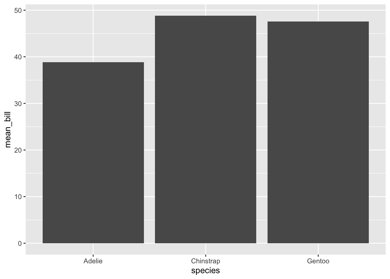
penguins %>% na.omit() %>% group_by(year, species) %>% summarize(mean = mean(bill_length_mm)) %>% ggplot(., aes(x = year, fill = species, y = mean)) + geom_col(position = "dodge")## `summarise()` has grouped output by 'year'. You can override using the
## `.groups` argument.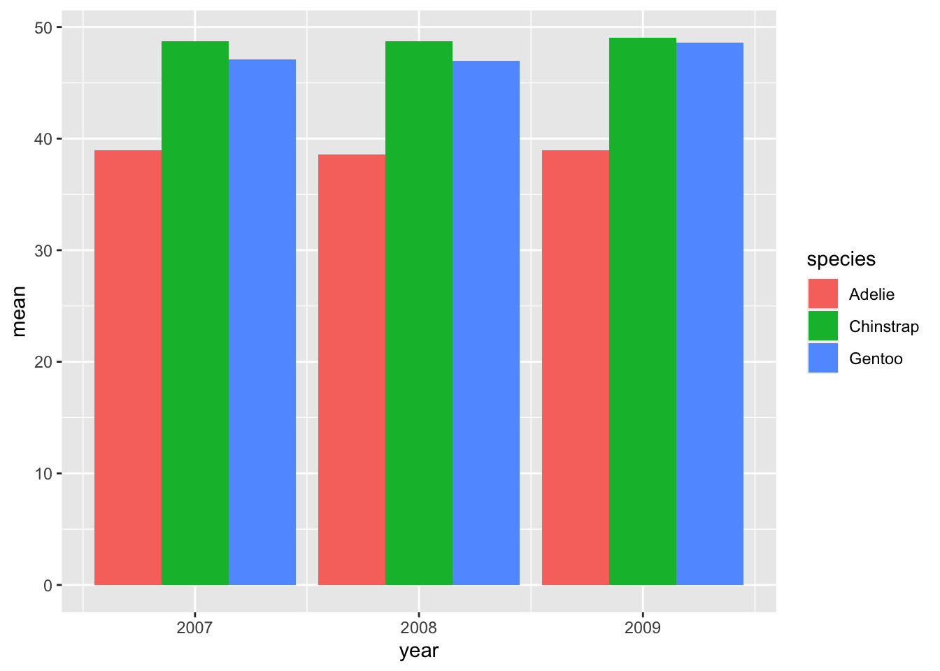
Practice
Try plotting the number of penguins on each island with a fill color by sex.
#Use geom_bar() to plot the counts
penguins %>%
  na.omit() %>%
  ggplot(., aes(x = island, fill = sex)) +
  geom_bar(position = "dodge")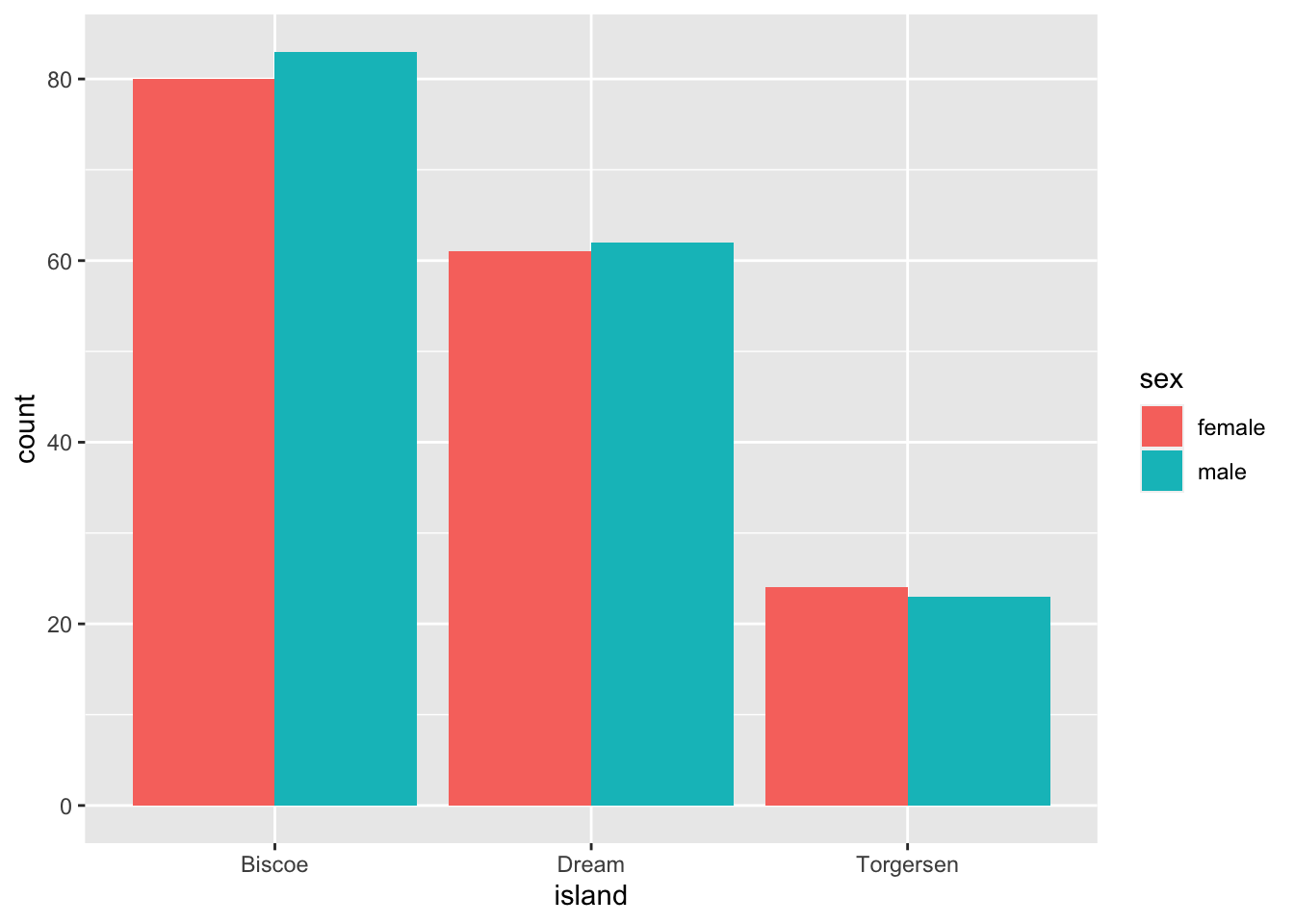
Next, plot the mean flipper length of each species, colored by sex
#Find the average flipper length by grouping by species and sex, then summarizing
penguins %>%
  group_by(species, sex) %>%
  na.omit() %>%
  summarize(mean_flipper_length = mean(flipper_length_mm)) %>%
#Use geom_col() to plot the average flipper length
  ggplot(., aes( x = species, y = mean_flipper_length, fill = sex)) +
  geom_col(position = "dodge")
## `summarise()` has grouped output by 'species'. You can override using the
## `.groups` argument.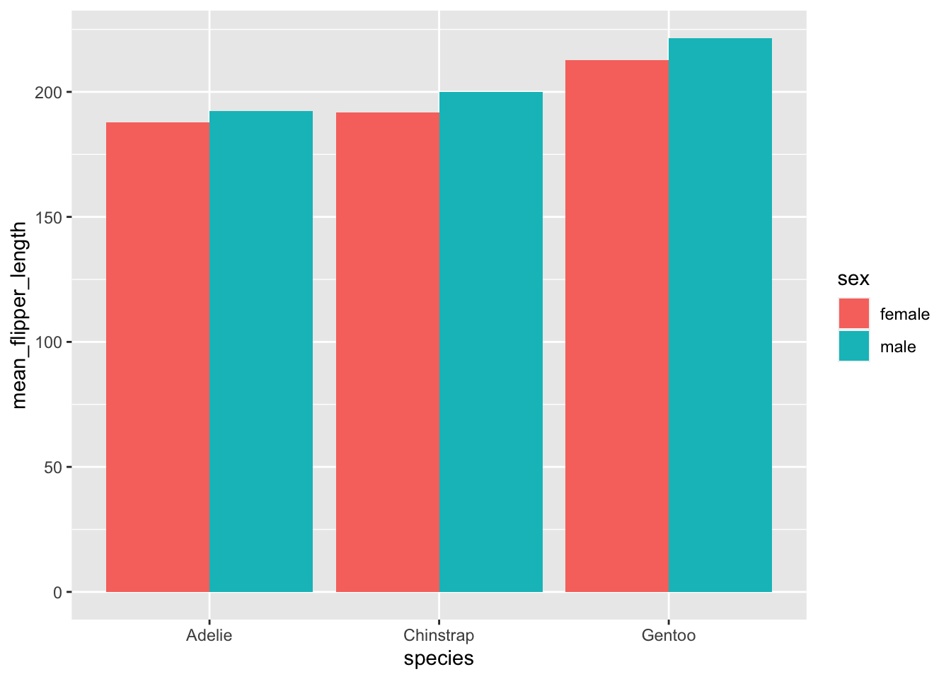
Boxplots
We often want to plot the statistics of our graphs, and box plots are one easy way to show the quantiles without doing a ton of work on adding error bars (which have more settings to include). The function is geom_boxplot().
#The basic plot structure
penguins %>% ggplot(., aes(x = species, y = flipper_length_mm)) + geom_boxplot()
## Warning: Removed 2 rows containing non-finite values (stat_boxplot).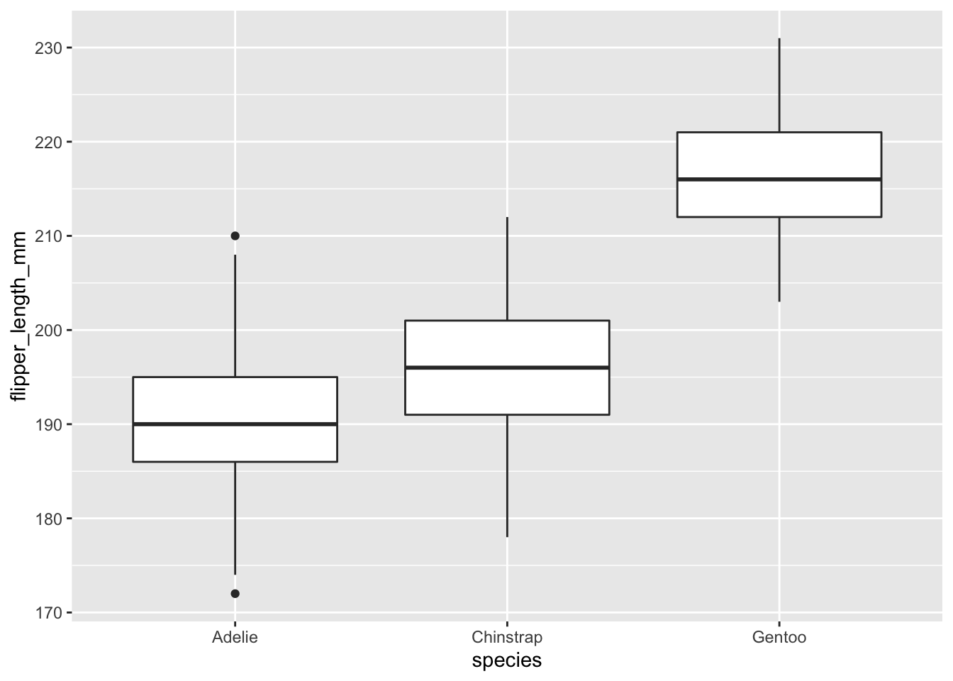
#Can you add in color by species? What happens if you color by sex?
penguins %>% ggplot(., aes(x = species, y = flipper_length_mm, color = species)) + geom_boxplot()
## Warning: Removed 2 rows containing non-finite values (stat_boxplot).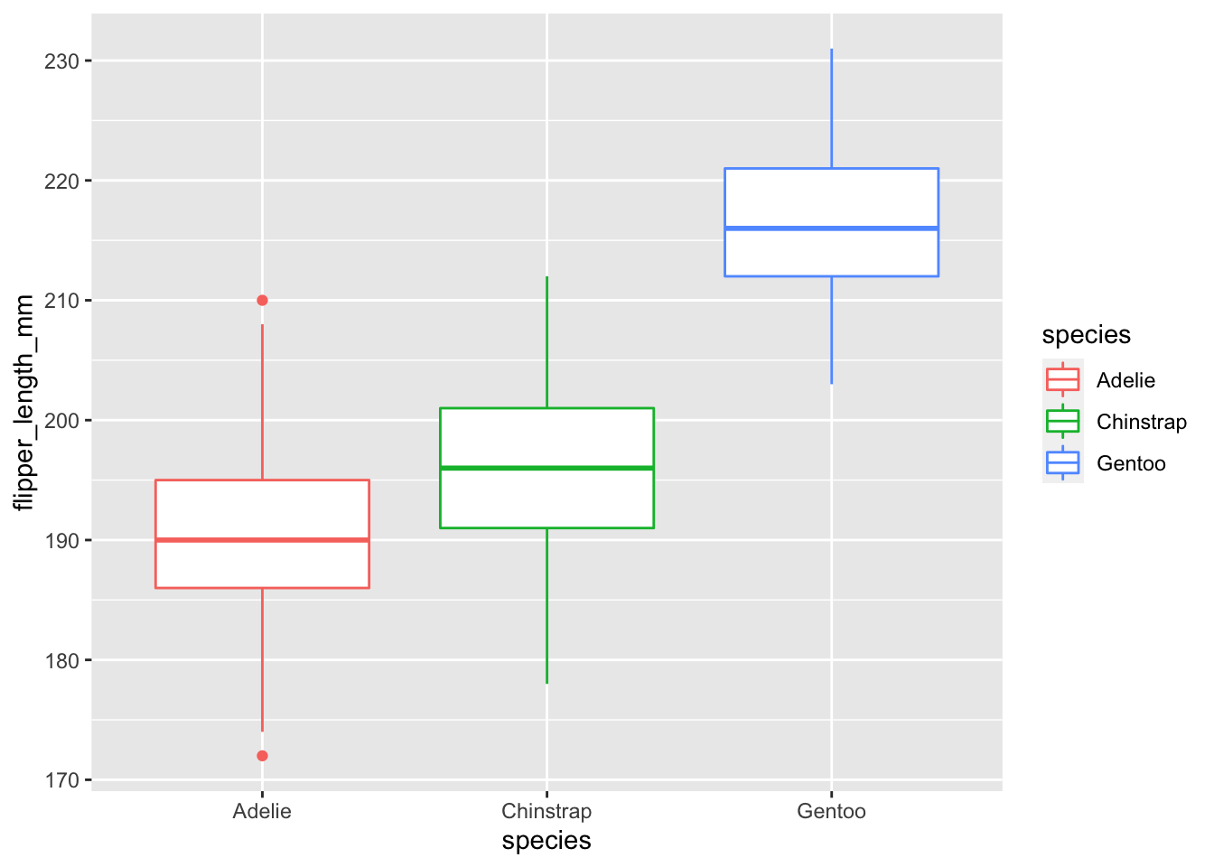
penguins %>% ggplot(., aes(x = species, y = flipper_length_mm, color = sex)) + geom_boxplot()## Warning: Removed 2 rows containing non-finite values (stat_boxplot).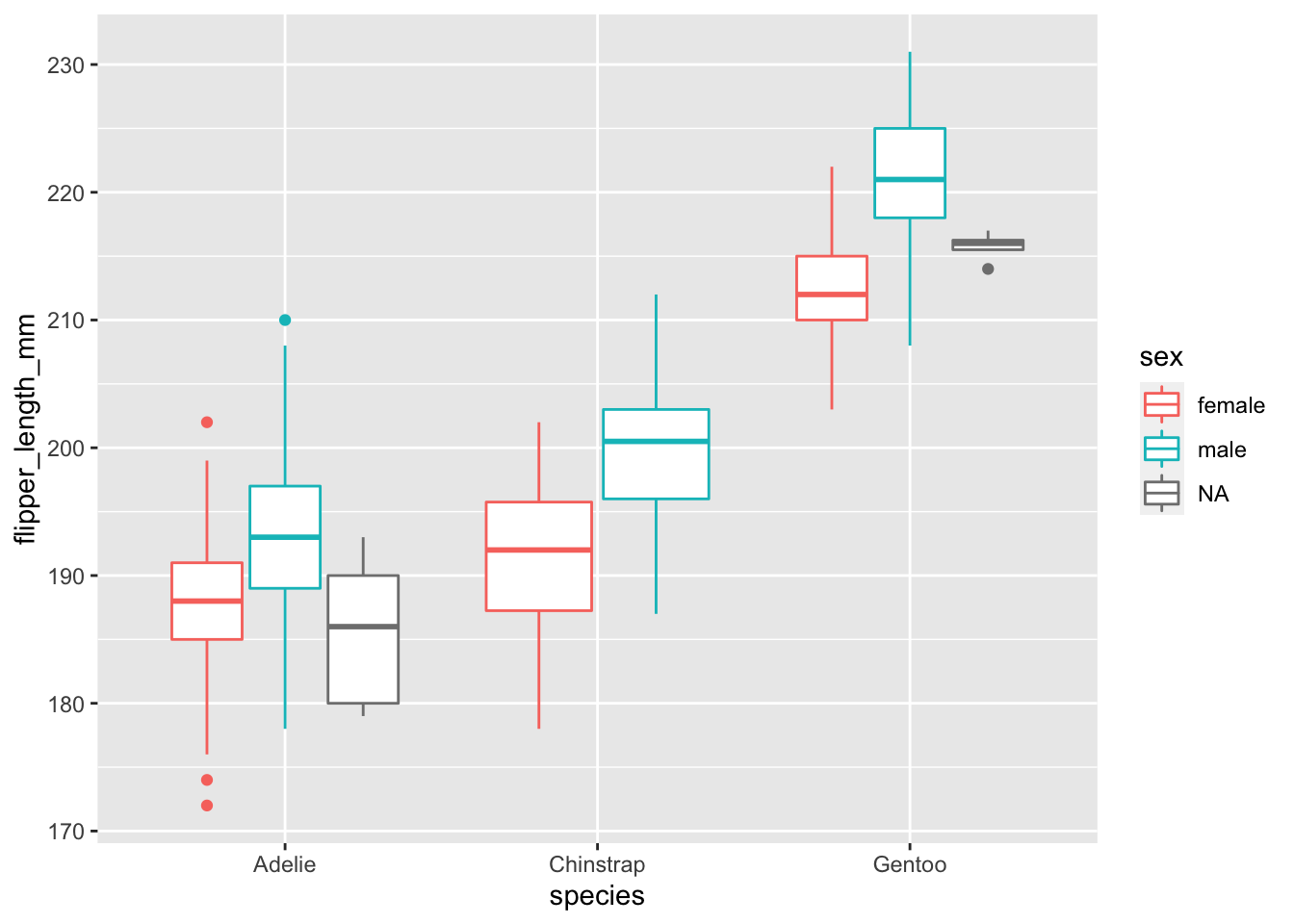
Practice
Change the above graph to remove NAs.
penguins %>%
  na.omit() %>%
  ggplot(., aes(x = species, y = flipper_length_mm, color = sex)) + geom_boxplot()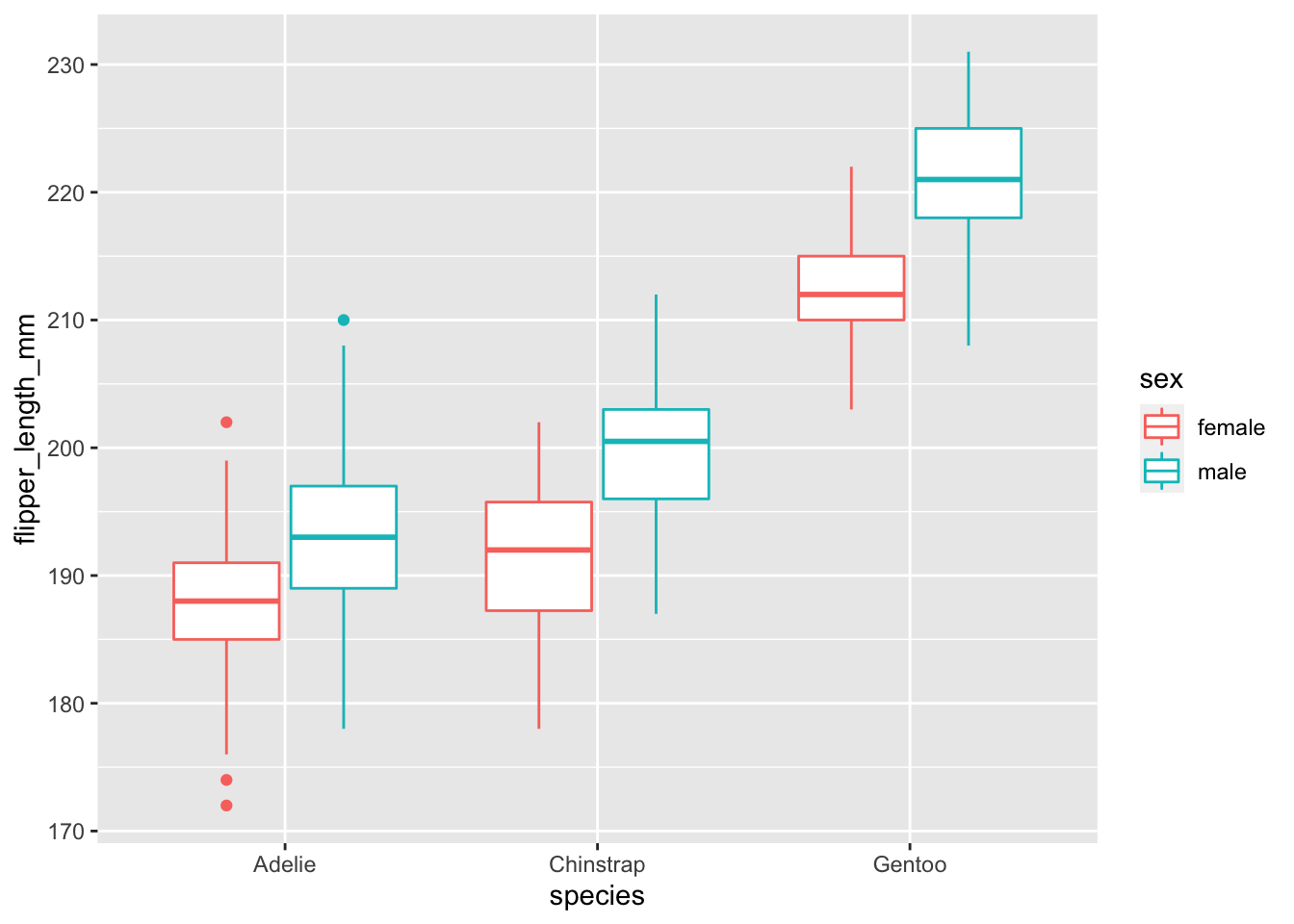
Plot the bill length instead of the flipper length.
penguins %>%
  na.omit() %>%
  ggplot(., aes(x = species, y = bill_length_mm, color = sex)) + geom_boxplot()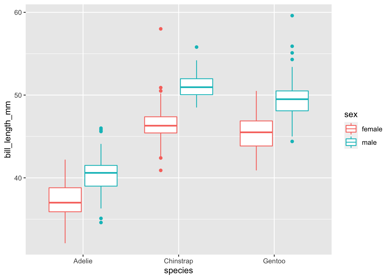
Exercises with new data
Let’s load a new csv to practice our plotting. This is from Cassandra’s data, and includes chromosomes, positions, and reads.
BSA_Reads <- read.csv("BSA_Reads.csv")#Look at the structure of iris to find what the options are for column names
str(BSA_Reads)## 'data.frame': 398312 obs. of 11 variables:
## $ X : int 1 2 3 4 5 6 7 8 9 10 ...
## $ CHROM : chr "I" "I" "I" "I" ...
## $ POS : int 100007 100007 100007 100007 100007 100007 100007 100007 1035 1035 ...
## $ value : int 867 590 815 160 86 189 322 43 137 99 ...
## $ allele: chr "ALT" "REF" "ALT" "REF" ...
## $ bulk : chr "HIGH" "LOW" "LOW" "LOW" ...
## $ parent: chr "Wine" "Oak" "Wine" "Wine" ...
## $ REF : chr "AT" "AT" "AT" "AT" ...
## $ Wine : chr "A" "A" "A" "A" ...
## $ Oak : chr NA NA NA NA ...
## $ Type : chr "Wine" "Wine" "Wine" "Wine" ...#What is the distribution of values? Use geom_density()
BSA_Reads %>%
ggplot(., aes(x = value)) +
geom_density()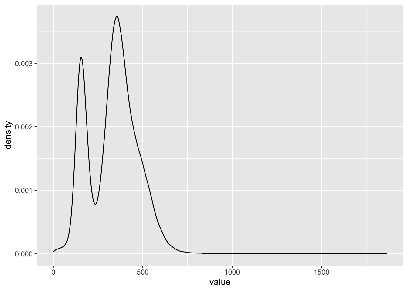
# How does the distribution differ with respect to parent? Use geom_density() but color by parent.
BSA_Reads %>%
  ggplot(., aes(x = value, color = parent)) +
  geom_density()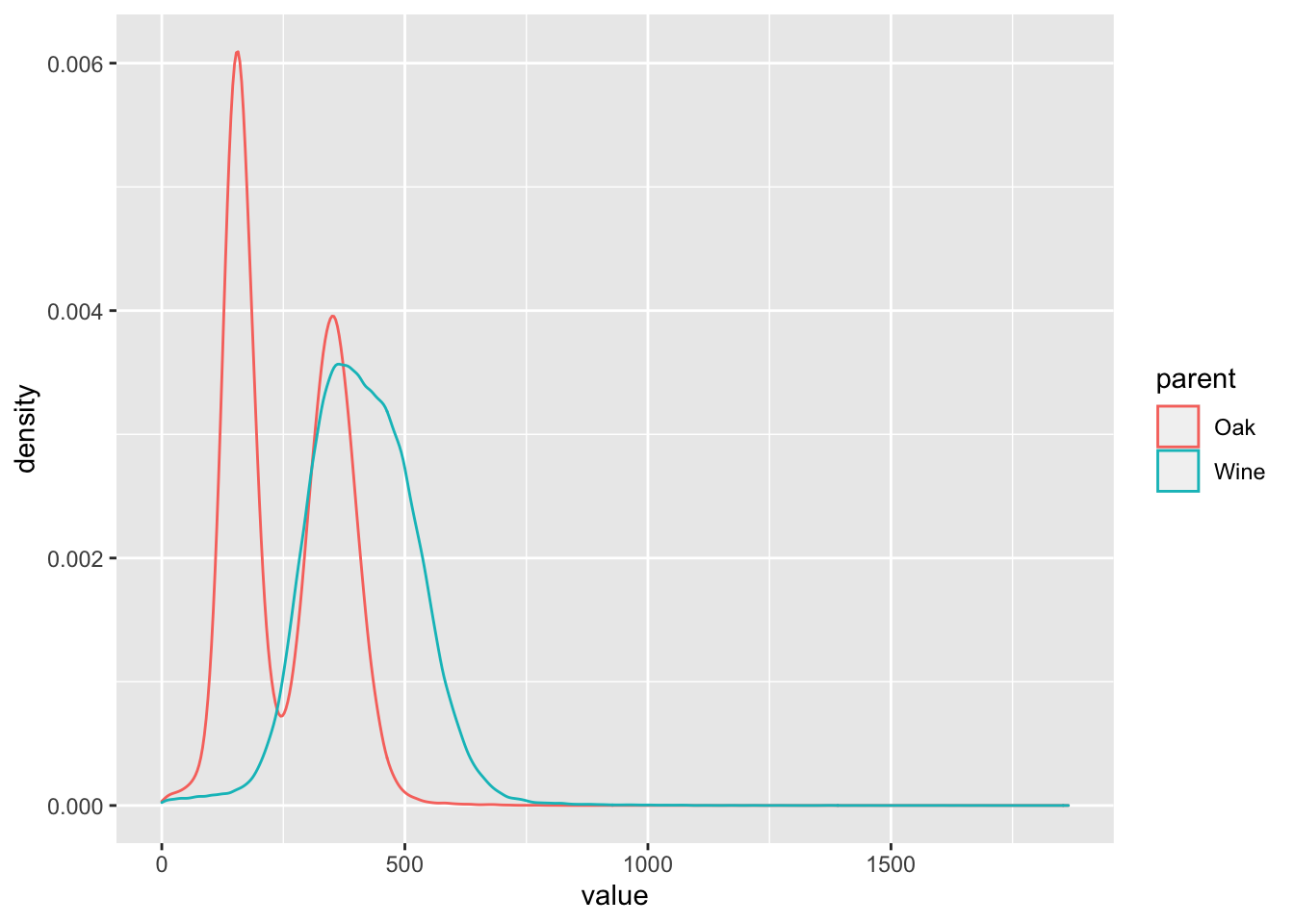
Let’s look at the average number of reads (value) for each bulk, colored by parent
# First, group by your bulk and parent
BSA_Reads %>%
  group_by(bulk, parent) %>%
#Next, use summarize to find the mean of the value
  summarize(avg_value = mean(value)) %>%
#Finally, plot using geom_col() with bulk as your x axis label, y as the mean of your reads, and a fill color of the parent
  ggplot(., aes(x = bulk, y = avg_value, fill = parent)) +
  geom_col() +
  xlab("Bulk") +
  ylab("Mean of Reads")
## `summarise()` has grouped output by 'bulk'. You can override using the
## `.groups` argument.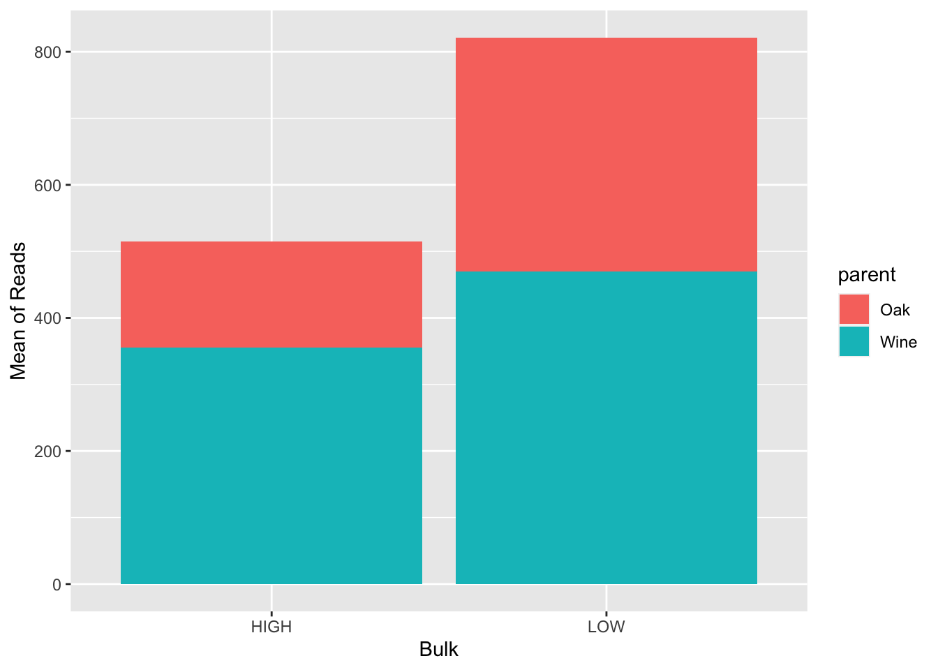
# Separate your plot so that the position is dodge (so that the bars are next to each other)
BSA_Reads %>%
  group_by(bulk, parent) %>%
#Next, use summarize to find the mean of the value
  summarize(avg_value = mean(value)) %>%
#Finally, plot using geom_col() with bulk as your x axis label, y as the mean of your reads, and a fill color of the parent
  ggplot(., aes(x = bulk, y = avg_value, fill = parent)) +
  geom_col(position = "dodge") +
  xlab("Bulk") +
  ylab("Mean of Reads")
## `summarise()` has grouped output by 'bulk'. You can override using the
## `.groups` argument.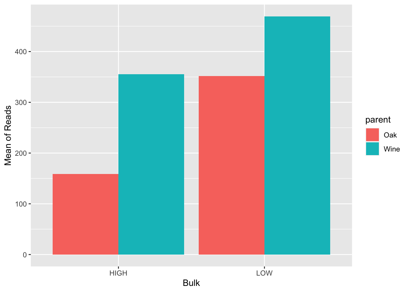
Finally, let’s look at the average value per chromosome, and the number of reads per chromosome.
#Use a boxplot to look at the values for each chromosome. Your x should be CHROM and y should be value.
BSA_Reads %>%
  ggplot(., aes(x = CHROM, y = value)) +
  geom_boxplot()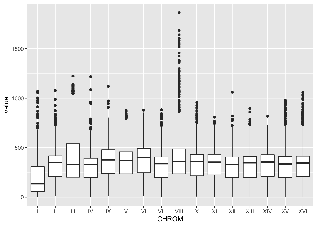
#Use geom_bar() for the number of entries for each chromosome. In this case you only need x to be CHROM since geom_bar() will count for you.
BSA_Reads %>%
  ggplot(., aes(x = CHROM)) +
  geom_bar()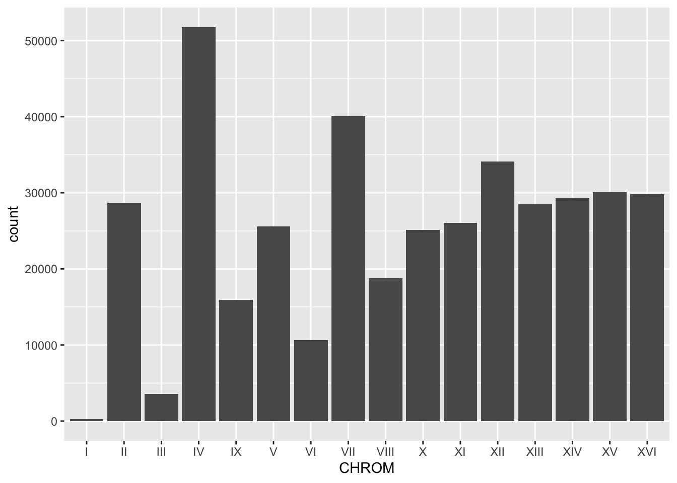
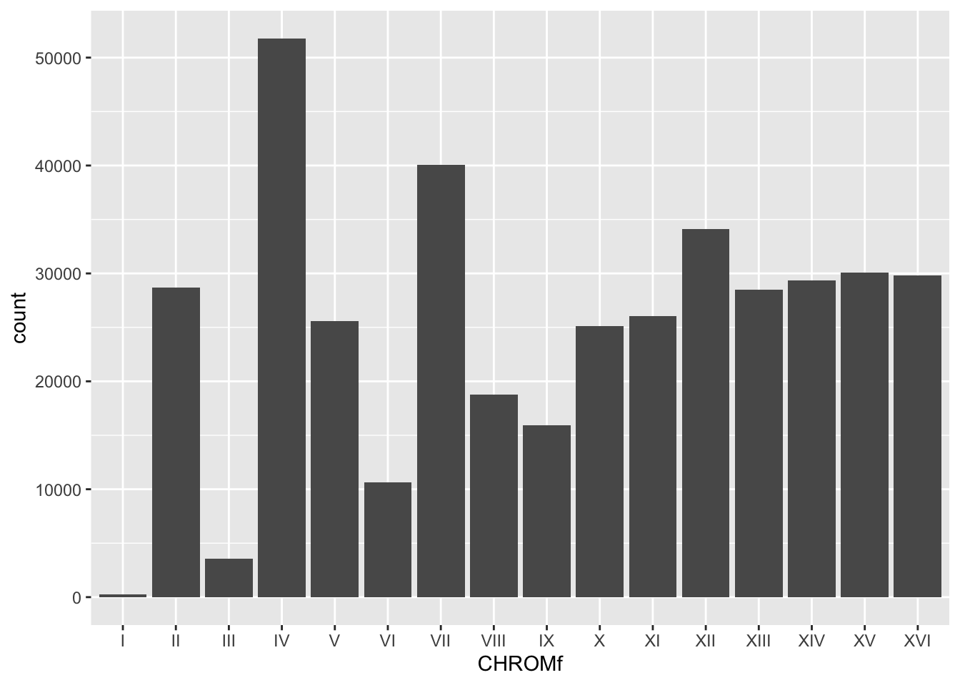
Bonus: Factors
The graphs of chromosomes are out of order, partially because they’re characters which are ordered alphabetically. However, Roman numerals don’t follow alphabetical order, so we can instead turn this column into a factor.
Factors have “levels” which determine their order. We can define this using factor(), just as we switched between numbers and characters.
BSA_Reads$CHROMf <- factor(BSA_Reads$CHROM,
                             levels = c("I", "II", "III", "IV", "V", "VI", "VII", "VIII",
                                        "IX", "X", "XI", "XII", "XIII", "XIV", "XV", "XVI"))

str(BSA_Reads)
## 'data.frame': 398312 obs. of 12 variables:
## $ X : int 1 2 3 4 5 6 7 8 9 10 ...
## $ CHROM : chr "I" "I" "I" "I" ...
## $ POS : int 100007 100007 100007 100007 100007 100007 100007 100007 1035 1035 ...
## $ value : int 867 590 815 160 86 189 322 43 137 99 ...
## $ allele: chr "ALT" "REF" "ALT" "REF" ...
## $ bulk : chr "HIGH" "LOW" "LOW" "LOW" ...
## $ parent: chr "Wine" "Oak" "Wine" "Wine" ...
## $ REF : chr "AT" "AT" "AT" "AT" ...
## $ Wine : chr "A" "A" "A" "A" ...
## $ Oak : chr NA NA NA NA ...
## $ Type : chr "Wine" "Wine" "Wine" "Wine" ...
## $ CHROMf: Factor w/ 16 levels "I","II","III",..: 1 1 1 1 1 1 1 1 1 1 ...Now, let’s plot this new variable as our x-axis.
BSA_Reads %>% ggplot(., aes(x = CHROMf)) + geom_bar()