Functions and Data Types

normalize_by_depth()

How do we define a function that normalize a vector of counts by total counts?

Before you start writing. Let’s start humble and get a small proportion of the data so you can capture errors right away when you test your function.

The key of doing this is to have something that you can tell whether your code is doing something you want right away with test data structurally similar to the real data.

# Take a small fraction of the data so we can test our function
test_count = head(rawcount)

Now, we are good to go. Let’s get the total count first!

# What is our input?
normalize_by_depth = function(input) {
  # How do we compute total count?
  
  # Let's divide everything by the total count calculated above
  
  # Provide an output
  
}

Let’s test the function with our naked eyes.

# Is the function doing what we expect it to do?
normalize_by_depth(test_count) == 1472 + 6 + 109 + 43

## logical(0)

If everything goes as expected, let’s divide everything by total count in the function, too.

# What is our input?
normalize_by_depth = function(input) {
  # How do we compute total count?
  depth = sum(input$count)
  # Let's divide everything by the total count calculated above
  
  # Provide an output
  # **Note that you would want to change your output!**
  return(depth)
}

Let’s test the revised function. What are we expecting here?

# We are expecting the first gene to be ~0.903 after normalization
# while the second gene is 0.
# Let's run the function on the test set and let the results print out.

Let’s multiply the result by \(10^{6}\) (10^6) before returning it in our function.

# What is our input?
normalize_by_depth = function(input) {
  # How do we compute total count?
  depth = sum(input$count)
  
  # Let's divide everything by the total count calculated above
  normalized_count = input$count/depth
  input$normalized_count = normalized_count
  
  # Provide an output
  return(input)
}

And test it again.

Note that for the first gene, we used to getting 0.9030675 before multiplying with \(10^{6}\).

normalize_by_depth(test_count)

##                   id count normalized_count
## 1 ENSMUSG00000000001  1472      0.903067485
## 2 ENSMUSG00000000003     0      0.000000000
## 3 ENSMUSG00000000028     6      0.003680982
## 4 ENSMUSG00000000031   109      0.066871166
## 5 ENSMUSG00000000037    43      0.026380368
## 6 ENSMUSG00000000049     0      0.000000000

get_tx_length()

A gene model file contains the starting and ending coordinates of genes, transcripts, and exons.

You can get a gene model file from Ensembl.

They are often stored as GTF/GFF3 files, but the format is beyond the scope of what we are going to do today. If you are interested, you can find more information about GTF/GFF format here.

# Load gene model file (pre-processed)
gene_model = read.csv("mouse_gene_model.csv")
head(gene_model)

##                   id     start       end
## 1 ENSMUSG00000102628 150956201 150958296
## 2 ENSMUSG00000100595 150983666 150984611
## 3 ENSMUSG00000097426 151012258 151012971
## 4 ENSMUSG00000097426 151013347 151013531
## 5 ENSMUSG00000104478 108344807 108347562
## 6 ENSMUSG00000104385   6980784   6981446

How do we define a function that get us lengths for each gene?

–

library(dplyr)

## 
## Attaching package: 'dplyr'

## The following objects are masked from 'package:stats':
## 
##     filter, lag

## The following objects are masked from 'package:base':
## 
##     intersect, setdiff, setequal, union

# How do we compute the length of each exons?
gene_model %>%
  head() %>%
  mutate(length = (end - start + 1))

##                   id     start       end length
## 1 ENSMUSG00000102628 150956201 150958296   2096
## 2 ENSMUSG00000100595 150983666 150984611    946
## 3 ENSMUSG00000097426 151012258 151012971    714
## 4 ENSMUSG00000097426 151013347 151013531    185
## 5 ENSMUSG00000104478 108344807 108347562   2756
## 6 ENSMUSG00000104385   6980784   6981446    663

Let’s test if the length column is correctly calculated.

# For the first gene
150958296 - 150956201   + 1

## [1] 2096

If it seems right, let’s get the sum of lengths per id now.

get_tx_length = function(input) {
  # How do we compute the sum of all exons of a gene?
  tx_length = input %>%
    mutate(length = (end - start + 1))
  # Group
  
  # Summarize by summation
  
  # Provide an output
  return(tx_length)
}

What does the output look like?

gene_model %>%
  head() %>%
  get_tx_length()

##                   id     start       end length
## 1 ENSMUSG00000102628 150956201 150958296   2096
## 2 ENSMUSG00000100595 150983666 150984611    946
## 3 ENSMUSG00000097426 151012258 151012971    714
## 4 ENSMUSG00000097426 151013347 151013531    185
## 5 ENSMUSG00000104478 108344807 108347562   2756
## 6 ENSMUSG00000104385   6980784   6981446    663

How do you independently test if the answer is correct for ENSMUSG00000097426?

# Doing it differently with base R
gene_of_interest = gene_model[gene_model$id == "ENSMUSG00000097426", ]
print(gene_of_interest)

##                   id     start       end
## 3 ENSMUSG00000097426 151012258 151012971
## 4 ENSMUSG00000097426 151013347 151013531

gene_of_interest$length = gene_of_interest$end - gene_of_interest$start + 1
print(gene_of_interest)

##                   id     start       end length
## 3 ENSMUSG00000097426 151012258 151012971    714
## 4 ENSMUSG00000097426 151013347 151013531    185

sum(gene_of_interest$length)

## [1] 899

How to merge data with a shared column?

If we check our small count table:

head(rawcount)

##                   id count
## 1 ENSMUSG00000000001  1472
## 2 ENSMUSG00000000003     0
## 3 ENSMUSG00000000028     6
## 4 ENSMUSG00000000031   109
## 5 ENSMUSG00000000037    43
## 6 ENSMUSG00000000049     0

and the first few rows of our gene length table:

gene_model %>%
  head() %>%
  get_tx_length()

##                   id     start       end length
## 1 ENSMUSG00000102628 150956201 150958296   2096
## 2 ENSMUSG00000100595 150983666 150984611    946
## 3 ENSMUSG00000097426 151012258 151012971    714
## 4 ENSMUSG00000097426 151013347 151013531    185
## 5 ENSMUSG00000104478 108344807 108347562   2756
## 6 ENSMUSG00000104385   6980784   6981446    663

You’ll see that we are almost done except that the row order are not exactly the same.

This can be taken care of by left_join(x, y, by = column), which is a dplyr function that **merge two data.frames (x and y) by a shared column.

(left_ means that it keeps all the rows in x even if y does not have it.)

Let’s see how it works. First, I’ll make a small table of gene length for testing.

test_gene_model = gene_model %>%
  # Only keep rows that are present in test_count
  filter(id %in% test_count$id)

# Compute gene length with our custom function
test_gene_length = test_gene_model %>% 
    get_tx_length()

print(test_gene_length)

##                    id     start       end length
## 1  ENSMUSG00000000037 159945768 159946244    477
## 2  ENSMUSG00000000037 159954486 159954531     46
## 3  ENSMUSG00000000037 159960243 159960313     71
## 4  ENSMUSG00000000037 159961033 159961267    235
## 5  ENSMUSG00000000037 159970260 159970348     89
## 6  ENSMUSG00000000037 159975200 159975443    244
## 7  ENSMUSG00000000037 159985010 159985093     84
## 8  ENSMUSG00000000037 159992191 159992265     75
## 9  ENSMUSG00000000037 159992605 159992679     75
## 10 ENSMUSG00000000037 159996237 159996320     84
## 11 ENSMUSG00000000037 159998176 159998259     84
## 12 ENSMUSG00000000037 160004662 160004745     84
## 13 ENSMUSG00000000037 160006153 160006236     84
## 14 ENSMUSG00000000037 160007457 160007540     84
## 15 ENSMUSG00000000037 160008873 160008956     84
## 16 ENSMUSG00000000037 160010369 160010452     84
## 17 ENSMUSG00000000037 160011673 160011756     84
## 18 ENSMUSG00000000037 160013087 160013170     84
## 19 ENSMUSG00000000037 160014396 160014479     84
## 20 ENSMUSG00000000037 160017609 160017692     84
## 21 ENSMUSG00000000037 160020476 160020753    278
## 22 ENSMUSG00000000037 160022746 160022860    115
## 23 ENSMUSG00000000037 160024984 160025187    204
## 24 ENSMUSG00000000037 160026362 160026544    183
## 25 ENSMUSG00000000037 160029253 160029363    111
## 26 ENSMUSG00000000037 160039562 160041192   1631
## 27 ENSMUSG00000000003  76897015  76897229    215
## 28 ENSMUSG00000000003  76891581  76891720    140
## 29 ENSMUSG00000000003  76888625  76888692     68
## 30 ENSMUSG00000000003  76886503  76886613    111
## 31 ENSMUSG00000000003  76886121  76886222    102
## 32 ENSMUSG00000000003  76885466  76885517     52
## 33 ENSMUSG00000000003  76881507  76881720    214
## 34 ENSMUSG00000000001 108053204 108053462    259
## 35 ENSMUSG00000000001 108031111 108031153     43
## 36 ENSMUSG00000000001 108030858 108030999    142
## 37 ENSMUSG00000000001 108025617 108025774    158
## 38 ENSMUSG00000000001 108023079 108023207    129
## 39 ENSMUSG00000000001 108019789 108019918    130
## 40 ENSMUSG00000000001 108019251 108019404    154
## 41 ENSMUSG00000000001 108016719 108016928    210
## 42 ENSMUSG00000000001 108014596 108016632   2037
## 43 ENSMUSG00000000031 142130566 142130647     82
## 44 ENSMUSG00000000031 142130350 142130484    135
## 45 ENSMUSG00000000031 142129268 142130267   1000
## 46 ENSMUSG00000000049 108286119 108286233    115
## 47 ENSMUSG00000000049 108286642 108286818    177
## 48 ENSMUSG00000000049 108288125 108288221     97
## 49 ENSMUSG00000000049 108295637 108295713     77
## 50 ENSMUSG00000000049 108298117 108298305    189
## 51 ENSMUSG00000000049 108299957 108300136    180
## 52 ENSMUSG00000000049 108302821 108303018    198
## 53 ENSMUSG00000000049 108305066 108305222    157
## 54 ENSMUSG00000000028  18630554  18630722    169
## 55 ENSMUSG00000000028  18630265  18630459    195
## 56 ENSMUSG00000000028  18630055  18630114     60
## 57 ENSMUSG00000000028  18629139  18629231     93
## 58 ENSMUSG00000000028  18627482  18627619    138
## 59 ENSMUSG00000000028  18626030  18626173    144
## 60 ENSMUSG00000000028  18624132  18624187     56
## 61 ENSMUSG00000000028  18620551  18620599     49
## 62 ENSMUSG00000000028  18617426  18617487     62
## 63 ENSMUSG00000000028  18616099  18616149     51
## 64 ENSMUSG00000000028  18614575  18614694    120
## 65 ENSMUSG00000000028  18613845  18613976    132
## 66 ENSMUSG00000000028  18613512  18613610     99
## 67 ENSMUSG00000000028  18611928  18612089    162
## 68 ENSMUSG00000000028  18605680  18605818    139
## 69 ENSMUSG00000000028  18605519  18605602     84
## 70 ENSMUSG00000000028  18603823  18603941    119
## 71 ENSMUSG00000000028  18603556  18603632     77
## 72 ENSMUSG00000000028  18600646  18600712     67
## 73 ENSMUSG00000000028  18599197  18599323    127

And… boom!

left_join(x = test_count, y = test_gene_length, by = "id")

##                    id count     start       end length
## 1  ENSMUSG00000000001  1472 108053204 108053462    259
## 2  ENSMUSG00000000001  1472 108031111 108031153     43
## 3  ENSMUSG00000000001  1472 108030858 108030999    142
## 4  ENSMUSG00000000001  1472 108025617 108025774    158
## 5  ENSMUSG00000000001  1472 108023079 108023207    129
## 6  ENSMUSG00000000001  1472 108019789 108019918    130
## 7  ENSMUSG00000000001  1472 108019251 108019404    154
## 8  ENSMUSG00000000001  1472 108016719 108016928    210
## 9  ENSMUSG00000000001  1472 108014596 108016632   2037
## 10 ENSMUSG00000000003     0  76897015  76897229    215
## 11 ENSMUSG00000000003     0  76891581  76891720    140
## 12 ENSMUSG00000000003     0  76888625  76888692     68
## 13 ENSMUSG00000000003     0  76886503  76886613    111
## 14 ENSMUSG00000000003     0  76886121  76886222    102
## 15 ENSMUSG00000000003     0  76885466  76885517     52
## 16 ENSMUSG00000000003     0  76881507  76881720    214
## 17 ENSMUSG00000000028     6  18630554  18630722    169
## 18 ENSMUSG00000000028     6  18630265  18630459    195
## 19 ENSMUSG00000000028     6  18630055  18630114     60
## 20 ENSMUSG00000000028     6  18629139  18629231     93
## 21 ENSMUSG00000000028     6  18627482  18627619    138
## 22 ENSMUSG00000000028     6  18626030  18626173    144
## 23 ENSMUSG00000000028     6  18624132  18624187     56
## 24 ENSMUSG00000000028     6  18620551  18620599     49
## 25 ENSMUSG00000000028     6  18617426  18617487     62
## 26 ENSMUSG00000000028     6  18616099  18616149     51
## 27 ENSMUSG00000000028     6  18614575  18614694    120
## 28 ENSMUSG00000000028     6  18613845  18613976    132
## 29 ENSMUSG00000000028     6  18613512  18613610     99
## 30 ENSMUSG00000000028     6  18611928  18612089    162
## 31 ENSMUSG00000000028     6  18605680  18605818    139
## 32 ENSMUSG00000000028     6  18605519  18605602     84
## 33 ENSMUSG00000000028     6  18603823  18603941    119
## 34 ENSMUSG00000000028     6  18603556  18603632     77
## 35 ENSMUSG00000000028     6  18600646  18600712     67
## 36 ENSMUSG00000000028     6  18599197  18599323    127
## 37 ENSMUSG00000000031   109 142130566 142130647     82
## 38 ENSMUSG00000000031   109 142130350 142130484    135
## 39 ENSMUSG00000000031   109 142129268 142130267   1000
## 40 ENSMUSG00000000037    43 159945768 159946244    477
## 41 ENSMUSG00000000037    43 159954486 159954531     46
## 42 ENSMUSG00000000037    43 159960243 159960313     71
## 43 ENSMUSG00000000037    43 159961033 159961267    235
## 44 ENSMUSG00000000037    43 159970260 159970348     89
## 45 ENSMUSG00000000037    43 159975200 159975443    244
## 46 ENSMUSG00000000037    43 159985010 159985093     84
## 47 ENSMUSG00000000037    43 159992191 159992265     75
## 48 ENSMUSG00000000037    43 159992605 159992679     75
## 49 ENSMUSG00000000037    43 159996237 159996320     84
## 50 ENSMUSG00000000037    43 159998176 159998259     84
## 51 ENSMUSG00000000037    43 160004662 160004745     84
## 52 ENSMUSG00000000037    43 160006153 160006236     84
## 53 ENSMUSG00000000037    43 160007457 160007540     84
## 54 ENSMUSG00000000037    43 160008873 160008956     84
## 55 ENSMUSG00000000037    43 160010369 160010452     84
## 56 ENSMUSG00000000037    43 160011673 160011756     84
## 57 ENSMUSG00000000037    43 160013087 160013170     84
## 58 ENSMUSG00000000037    43 160014396 160014479     84
## 59 ENSMUSG00000000037    43 160017609 160017692     84
## 60 ENSMUSG00000000037    43 160020476 160020753    278
## 61 ENSMUSG00000000037    43 160022746 160022860    115
## 62 ENSMUSG00000000037    43 160024984 160025187    204
## 63 ENSMUSG00000000037    43 160026362 160026544    183
## 64 ENSMUSG00000000037    43 160029253 160029363    111
## 65 ENSMUSG00000000037    43 160039562 160041192   1631
## 66 ENSMUSG00000000049     0 108286119 108286233    115
## 67 ENSMUSG00000000049     0 108286642 108286818    177
## 68 ENSMUSG00000000049     0 108288125 108288221     97
## 69 ENSMUSG00000000049     0 108295637 108295713     77
## 70 ENSMUSG00000000049     0 108298117 108298305    189
## 71 ENSMUSG00000000049     0 108299957 108300136    180
## 72 ENSMUSG00000000049     0 108302821 108303018    198
## 73 ENSMUSG00000000049     0 108305066 108305222    157

This works regardless of how the rows are ordered. You can try messing up the rows and see how if it makes a difference.

# Mess up the rows and do left_join() again.
# Say we have test_count[c(1, 3, 5, 2, 4, 6), ] and
# test_gene_model[c(6, 5, 4, 3, 2, 1), ]

One function to do it all

You must have noticed that functions are like Russian dolls: There are always functions inside a function.

Now that we have normalize_by_depth to generate CPM, get_tx_length to calculate gene length, and we know that left_join can merge them by ID, we can write a master function to streamline everything.

normalize_rnaseq = function(count, gene_model){
  # 1. Normalize read counts by sequencing depth = total reads we got from a sample.
  # (This gives CPM)

  # 2. Normalize again with transcript length.
  # (CPM/Gene length = Transcript per million (TPM))
  
  # 3. Make a master table containing both CPM and length per gene

  return(normalized_count)
}

Finally, let’s test it:

normalize_rnaseq(test_count, test_gene_model)

## Error in normalize_rnaseq(test_count, test_gene_model): could not find function "normalize_rnaseq"

All your hard work pays now – you can normalize the whole thing with ease!

# Normalize the full table with full gene model

characters are friendly most of the time, but…

# There's a L0 masquerading as 10 in your csv!
fake_num = c("1", "3", "5", "7", "9", "l0")

typeof(fake_num)

## [1] "character"

as.numeric(fake_num)

## Warning: NAs introduced by coercion

## [1]  1  3  5  7  9 NA

chr_vec = c("5", "8", "6", "10", "7", "9")

# You might not expect it to sort like this
sort(chr_vec)

## [1] "10" "5"  "6"  "7"  "8"  "9"

# If they are numbers, they sort differently
sort(as.numeric(chr_vec))

## [1]  5  6  7  8  9 10

Numeric type: Precision can be dangerous…

0.1 + 0.2 == 0.3

## [1] FALSE

There’s a website called https://0.30000000000000004.com/ that explains this in detail.

But briefly, any number that is not an integer has limited precision, and propagation of error is a thing.

# A more robust way to compare non-integers
# Define an error margin that you want to tolerate
error_margin = 10^-8

# and then decide if the difference is within the margin
(0.1 + 0.2) - 0.3 < error_margin

## [1] TRUE

Factor: Ordered categories

# Categories as characters works most of the time, but...
month_tbl = data.frame(
  month = c(
    "January", "February", "March", "April", "May", "June",
    "July", "August", "September", "October", "November", "December"
  ),
  length = c(
    31, 28, 31, 30, 31, 30, 31, 31, 30, 31, 30, 31
  )
)
str(month_tbl)

## 'data.frame':    12 obs. of  2 variables:
##  $ month : chr  "January" "February" "March" "April" ...
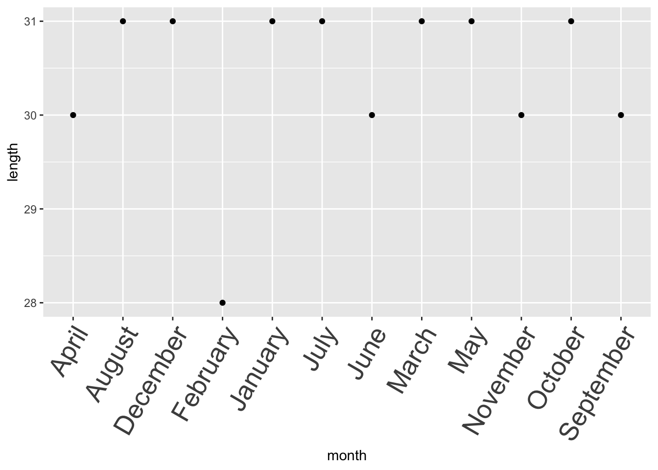
##  $ length: num  31 28 31 30 31 30 31 31 30 31 ...

Most functions that you encounter in R will sort alphabetically for characters.

library(ggplot2)
month_tbl %>%
  qplot(data = ., x = month, y = length, geom = "point") +
  # This adjust the axis text to make the text more visible
  theme(axis.text.x = element_text(size = 20, angle = 60, hjust = 1))

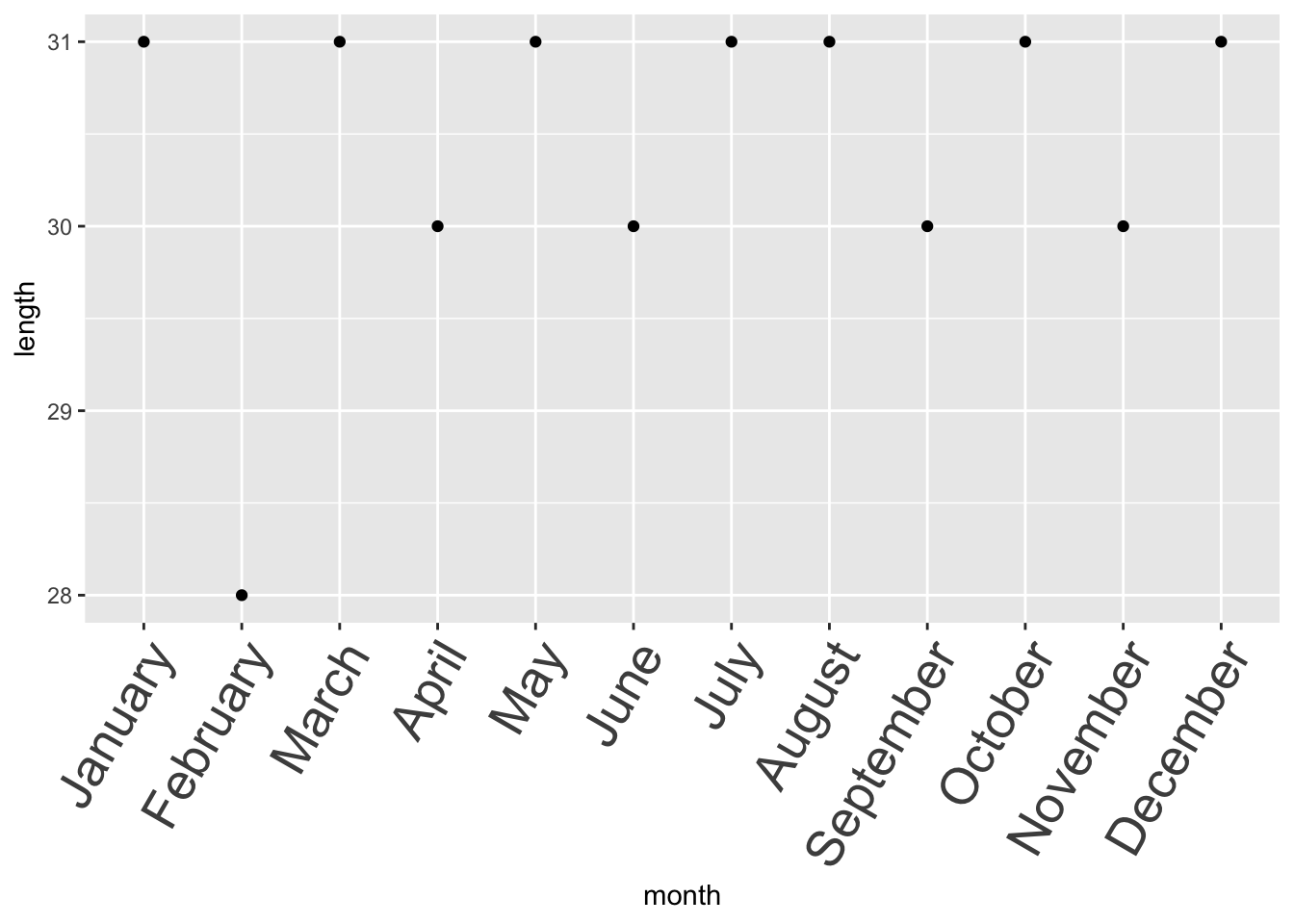
You won’t be able to decide the order unless you convert it to a factor.

month_tbl$month = factor(
  month_tbl$month,
  # R will respect the levels you set here
  levels = c(
    "January", "February", "March", "April", "May", "June",
    "July", "August", "September", "October", "November", "December"
  )
)

month_tbl %>%
  qplot(data = ., x = month, y = length, geom = "point") +
  # This adjust the axis text to make the text more visible
  theme(axis.text.x = element_text(size = 20, angle = 60, hjust = 1))

Factors are more complicated than characters and numbers, so they could be harder to troubleshoot, but at the same time, they are very powerful especially in statistics.

As a rule of thumb, when you inspect your data (e.g., with str()), always ask yourself if you are having categorical variables.

If you do, consider converting them to factors if:

• You know they are ordinal

• When you are building statistical models with categorical variables (ANOVA et al.)

Date and time

They have a similar issue as ordinal categories: If considered as characters, they won’t be ordered chronologically.

# This shouldn't be surprising by now
random_dates = c("12-25-2022", "07-04-1989", "01-01-2077")
sort(random_dates)

## [1] "01-01-2077" "07-04-1989" "12-25-2022"

Unlike most categorical variables, there are usually so many dates, so it is not practical for you to assign orders manually.

Luckily, there is a package that will take care of this for you if you tell it the format of your dates.

# You can tell R how the date is represented to chronologically sort
library(lubridate)

## 
## Attaching package: 'lubridate'

## The following objects are masked from 'package:base':
## 
##     date, intersect, setdiff, union

# mdy() stands for month, day, year
good_dates = mdy(random_dates)
sort(good_dates)

## [1] "1989-07-04" "2022-12-25" "2077-01-01"