Understanding Functions
Review
Let’s create our data frames again by running the following code:
NewDataFrame <- data.frame(Random = c(4, 20, 10, 21, 63, 3, 14, 60, 9, 6),
                           Index = 1:10,
                           Categories = c("Month", "Day", "Month", "Day", "Year",
                                          "Month", "Day", "Year", "Month", "Day"))
Examples for plotting subsetted values
If you wanted to plot only specific values, you could use these same booleans inside the functions to plot. This is going to be the basis of how we separate out values in our plots.
library(ggplot2)
library(dplyr)
##
## Attaching package: 'dplyr'## The following objects are masked from 'package:stats':
##
## filter, lag## The following objects are masked from 'package:base':
##
## intersect, setdiff, setequal, union# Plot our data frame here
qplot(x = NewDataFrame$Random, y = NewDataFrame$Index)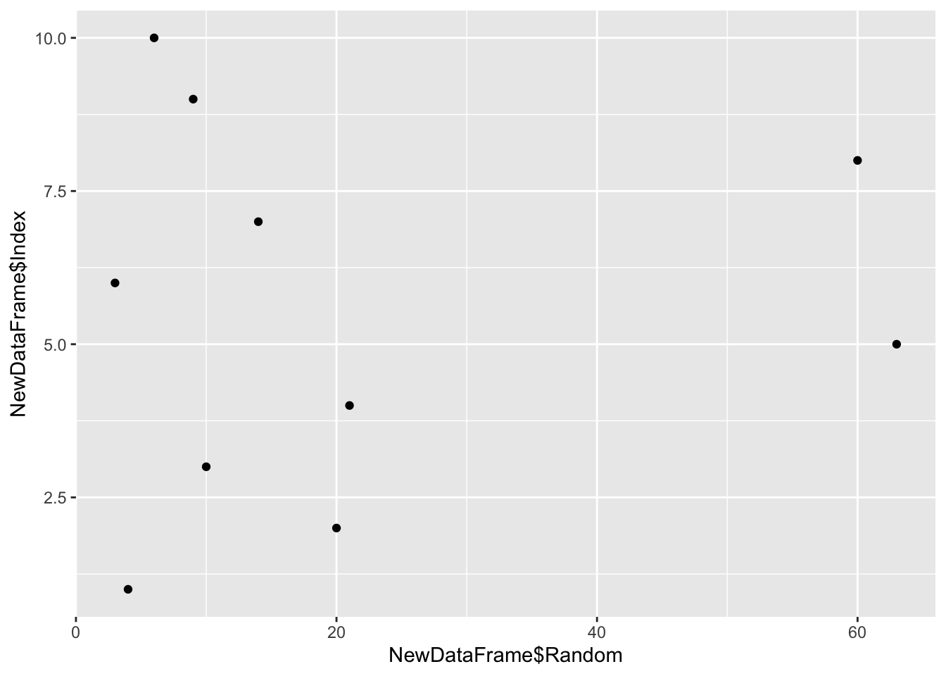
qplot(x = Random, y = Index, data = NewDataFrame)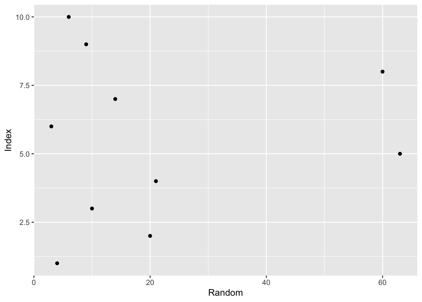
# We can change the size of our points by adding in the 'size' argument
qplot(x = NewDataFrame$Random, y = NewDataFrame$Index, size = 1)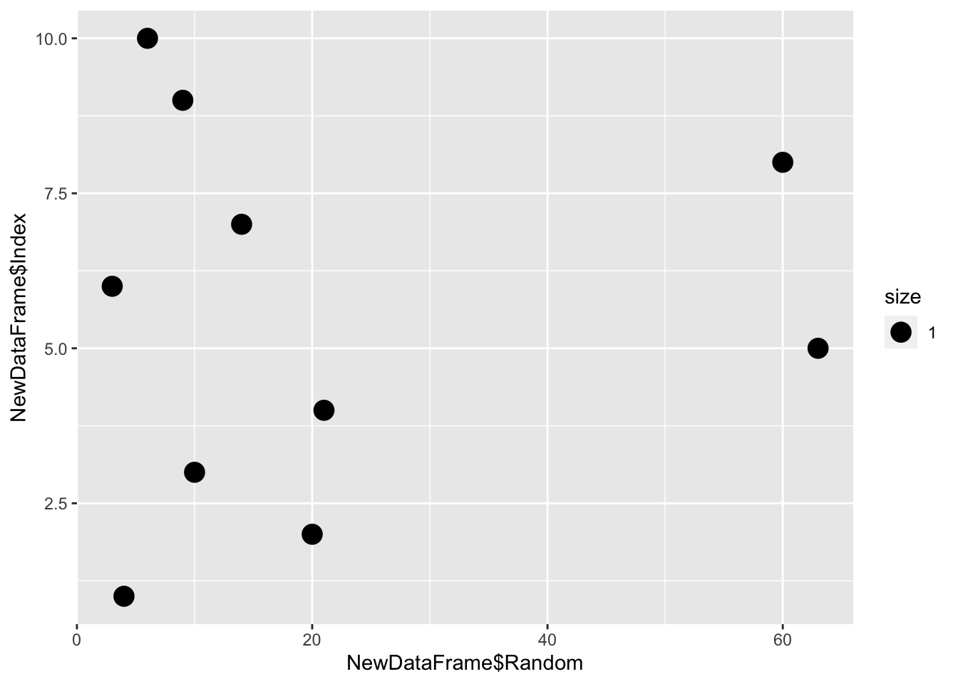
# Finally, we can add in coloring by a boolean logical
qplot(x = NewDataFrame$Random, y = NewDataFrame$Index, color = NewDataFrame$Index > 5, size = 1)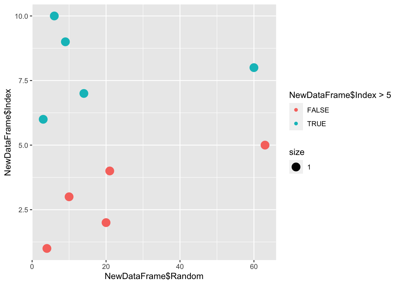
qplot(x = NewDataFrame$Random, y = NewDataFrame$Index, color = NewDataFrame$Categories, size = 1)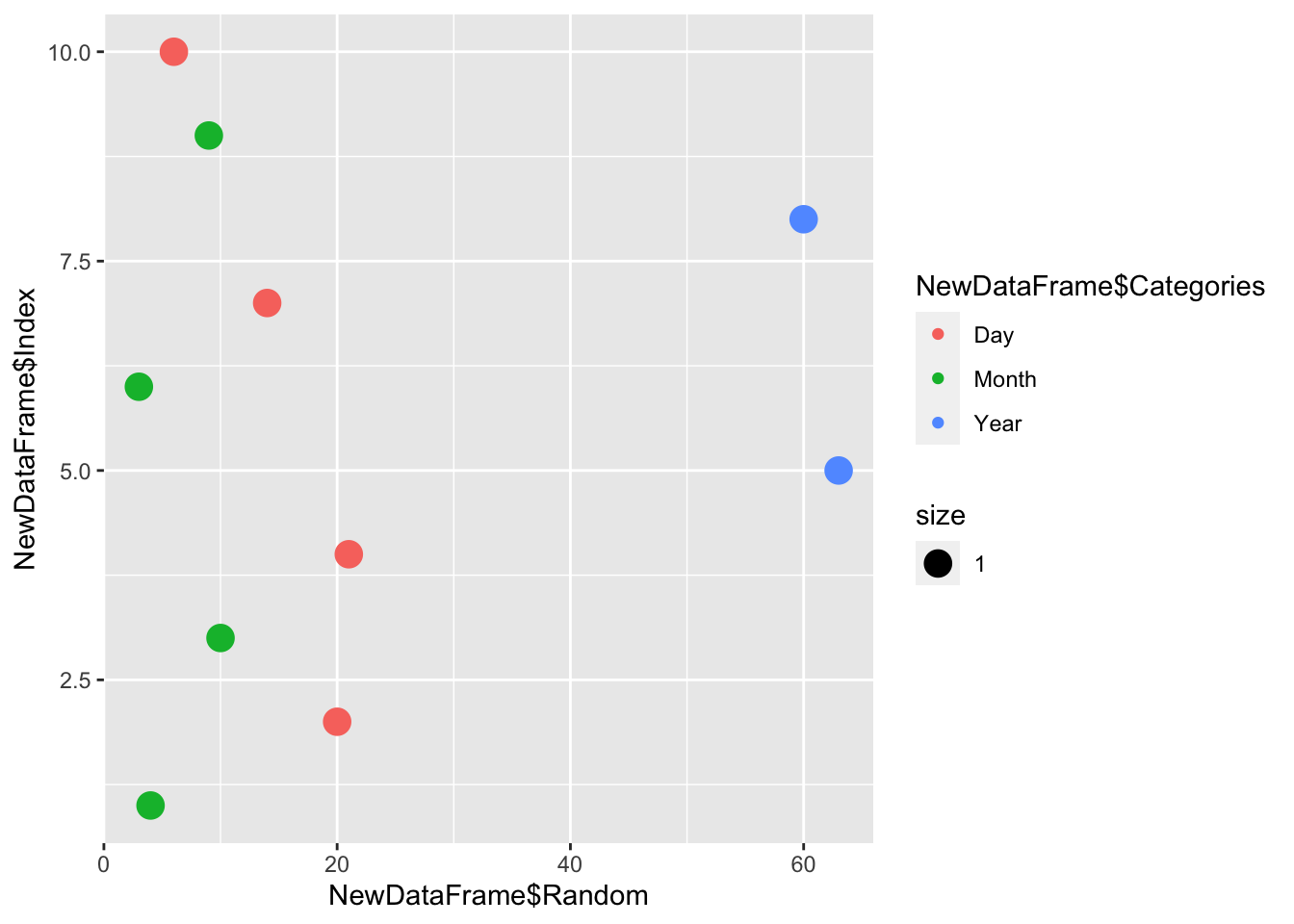
Exploring R
As a reminder, we can find out more about the functions we use with the help menu, found using help() or just simply a ‘?’ in front of the function (without spaces).
help(qplot)
?qplot
As a reminder, there’s an option for geom. This is the type of plot that will be made, and the default is a scatter plot (so geom = “point”). You can find this in the defaults for geom.
#Make a scatter plot
qplot(x = Index, y = Random, data = NewDataFrame,
      geom = "point",
      xlim = c(0,25), ylim = c(0,100),
      main = "Rainfall Distribution",
      xlab = "Month",
      ylab = "Rainfall (in)",
      color = Random > 5, size = 1)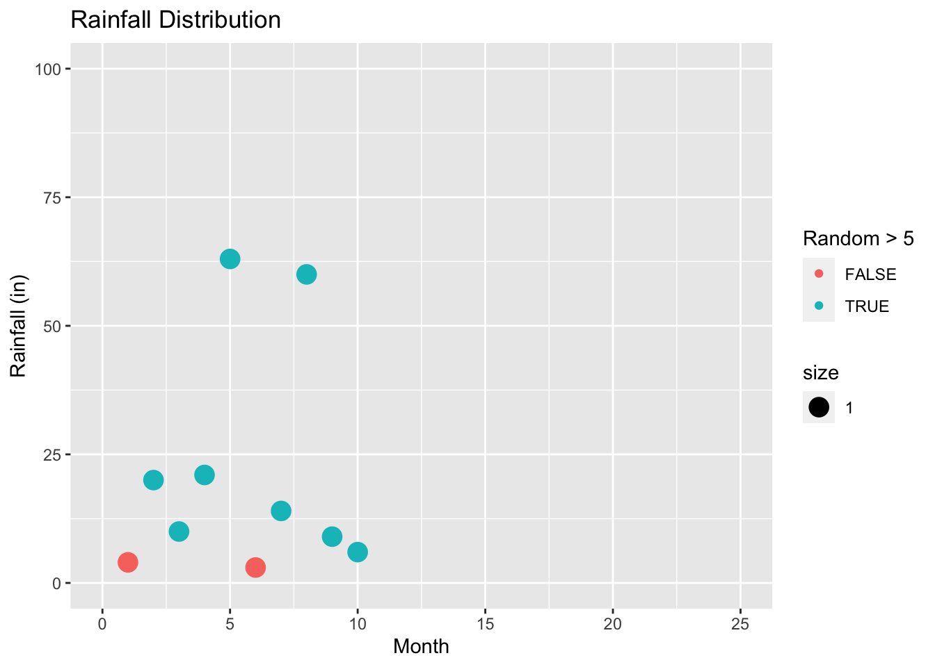
#Make a box plot with scatter (called jitter)
qplot(x = Random, y = Categories, data = NewDataFrame,
      geom = c("boxplot", "jitter"),
      main = "Boxplot of Random Numbers",
      color = Index)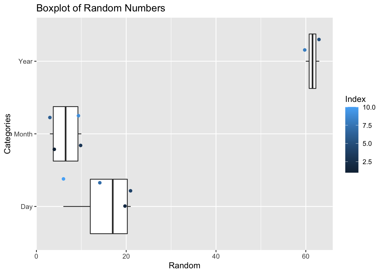
Practice from last time:
Load in the dataset penguins.csv, and plot the bill length vs body mass of penguins, coloring by species and changing the shape by island.
#Load in the csv using read.csv()

#View the data by using head() and find the names of the columns using str()

#Use qplot to plot the columns that you're interested in
Advanced Practice
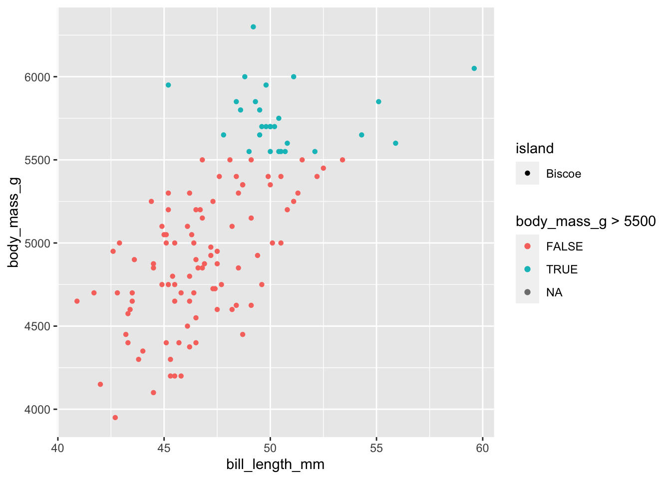
Using either dplyr or subsetting, plot the Gentoo penguins bill length vs body mass, and color by if their body mass is above 5500.
# Your code belowFunctions
We’ve been using functions throughout this course; a function is anything that has an input and an output, often changing that input to create a different output. The functions that we’ve used so far have either been built into R such as mean(), dim(), sum(), and length(), or they have been loaded in as a package, such as dplyr::filter(), dplyr::summarize(), and ggplot::qplot().
Let’s now look up the help menu for the function seq(). What does it do?
help(seq)Let’s run this function with default values:
#Uncomment this line to see what happens if you don't include any values:
#seq()

#Let's run this line to see what happens when you include only a single value:
seq(5)
## [1] 1 2 3 4 5Let’s include three numbers without explicitly calling each argument:
seq(5,10,2)## [1] 5 7 9#This is the same as running:
seq(from = 5, to = 10, by = 2)## [1] 5 7 9Let’s change up the order now:
#This will also produce values that are equivalent:
seq(to = 10, by = 2, from = 5)
## [1] 5 7 9#But this will not:
#seq(10, 2, 5)Practice
Save a vector of values from 12 to 200, increasing by 4. Then print the last 10 values of this vector.
#define your variable as the output of seq()

#look at the documentation for tail()

#print the last 10 values using tail()
Writing your own function
We can write functions as well as using them. Today we’ll start off with a simple code to convert Celsius to Fahrenheit.
#define your variable
celcius <- 20

#calculate your new value
farenheit <- 9/5 * celcius + 32

#print the new value
farenheit
## [1] 68Now let’s turn this into a function, using the function() function. Keep in mind that functions follow essentially the format of
\[y=f(x)\]
which can also be read as:
\[output = myfunction(input)\]
When we write this in code, we define the name of the function (below it’s c2f) as function(input){}, where inside the curly brackets {} there is the actual calculation. We then use the function return() to designate to the function what to output, which is our “y” in the above formula.
c2f <- function(celcius) {
  farenheit = 9/5 * celcius + 32
  return(farenheit)
}
What happens if we run this without an argument?
#Run the following code:
c2f()
We need to include arguments for celcius:
#Try explicitly stating the value
c2f(celcius = 10)
## [1] 50#What happens if we don't define celcius?
c2f(10)## [1] 50Finally, we can actually include a default when we create this function. Let’s add in something to c2f().
c2f_adv <- function(celcius = 0) {
  farenheit <- 9/5 * celcius + 32
  return(farenheit)
}

#now run the code without an argument to see what happens
c2f_adv()
## [1] 32Functions with two arguments:
If we include x and y into the equation, we can set two variables values:
multiply <- function(x, y){x*y}Now we can run this, but it won’t work if we don’t give two arguments:
#This does not work without defaults
#multiply()

#This will multiply 2 and 3:
multiply(2,3)
## [1] 6If we rewrite this function, then it will work if defaults are set:
multiply2 <- function(x = 2, y = 4){x*y}

#This will multiply the default arguments
multiply2()
## [1] 8#This will multiply the inputs
multiply2(3,10)## [1] 30#What happens if you only include one number?
multiply2(10)## [1] 40multiply2(y = 10)## [1] 20Data Types
So far we’ve been able to run calculations using variables, and used read.csv() to take in a character (the name of your file) that is converted into a data frame. We’ve also mentioned that data frame columns must be vectors of the same “type”. But what are the other data types that R can use?
Some basic data types:
Characters (char): “string” of text, which has the value of the text
Numbers (num): overall class of numbers, which includes integers and doubles
Integers (int): numbers without decimal points (takes less space)
Doubles (dbl): floating point numbers, or those with precision (takes more space)
Factors (fact): categorical elements which can be ordered (this sounds weird, but we’ll explain more later)
examplestring <- "This is a string of text"
exampledouble <- 26.2
exampleinteger <- 5

#We can find out the data types by running typeof()

typeof(examplestring)
## [1] "character"#What data types are exampledouble and exampleinteger?
typeof(exampledouble)## [1] "double"typeof(exampleinteger)## [1] "double"#Notice that exampleinteger is also listed as a double; this is because R will automatically store numbers as doubles, and converts between numeric classes automatically
realinteger <- as.integer(exampleinteger)
typeof(realinteger)## [1] "integer"When plotting, data types will change how plots view your data. For example, characters will often be unique values without order, numbers will often be continuous rather than discrete, and ordered alphabetically, and factors will be discrete and maintain an order. We will learn more about this soon, but we can use an example with qplot (which we’ve reviewed).
penguins <- read.csv("penguins.csv")
# How many colors are there when we color by island?
qplot(x = bill_length_mm, y = bill_depth_mm, data = penguins, color = island)
## Warning: Removed 2 rows containing missing values (geom_point).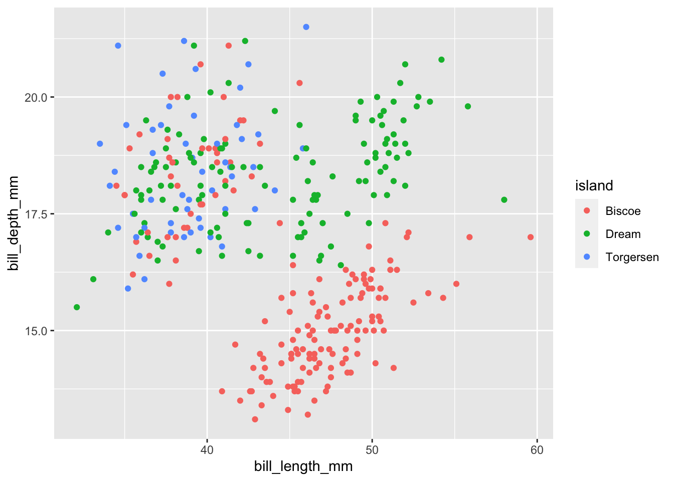
# How many colors are there when we color by bill depth?
qplot(x = bill_length_mm, y = bill_depth_mm, data = penguins, color = bill_depth_mm)
## Warning: Removed 2 rows containing missing values (geom_point).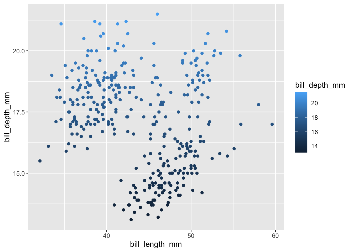
Answers to practice problems
## 'data.frame':    344 obs. of  8 variables:
##  $ species          : chr  "Adelie" "Adelie" "Adelie" "Adelie" ...
##  $ island           : chr  "Torgersen" "Torgersen" "Torgersen" "Torgersen" ...
##  $ bill_length_mm   : num  39.1 39.5 40.3 NA 36.7 39.3 38.9 39.2 34.1 42 ...
##  $ bill_depth_mm    : num  18.7 17.4 18 NA 19.3 20.6 17.8 19.6 18.1 20.2 ...
##  $ flipper_length_mm: int  181 186 195 NA 193 190 181 195 193 190 ...
##  $ body_mass_g      : int  3750 3800 3250 NA 3450 3650 3625 4675 3475 4250 ...
##  $ sex              : chr  "male" "female" "female" NA ...
##  $ year             : int  2007 2007 2007 2007 2007 2007 2007 2007 2007 2007 ...
## Warning: Removed 2 rows containing missing values (geom_point).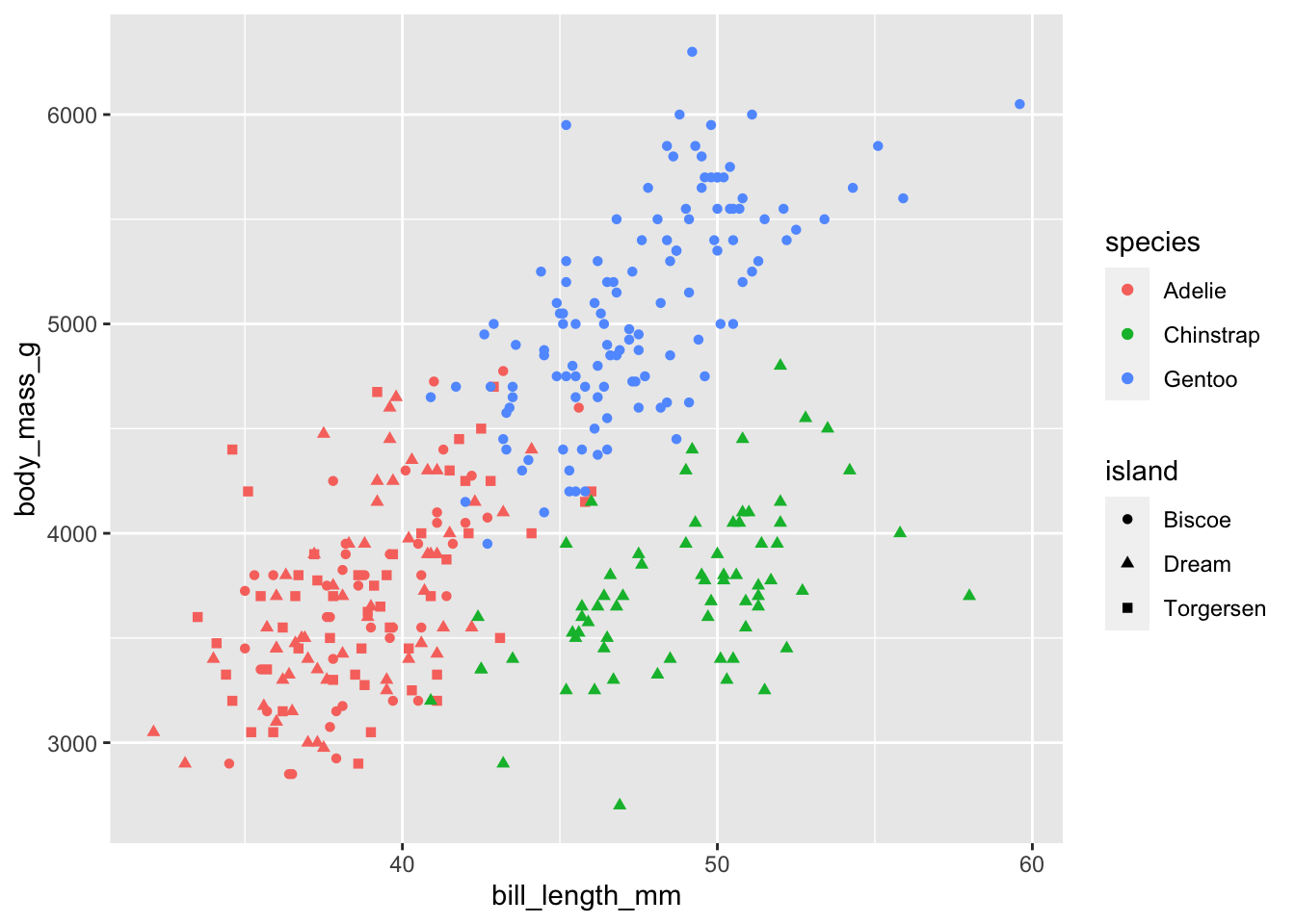
## Warning: Removed 1 rows containing missing values (geom_point).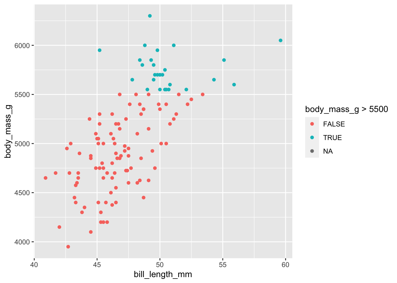
## Warning: Removed 1 rows containing missing values (geom_point).