Understanding Indexing and Subsetting
Indexing
What do we mean by indexing?
So far, we’ve worked with data frames in R. Each data frame is really a set of rows and columns with values populated, and these can be broken down into what are called vectors. A vector is simply a one-dimensional set of something that can have at minimum length 1.
We can create vectors using the function c(), for concatenate.
FirstVector <- c(4,20,10,21,60,3,14,63,9,6)

FirstVector
## [1] 4 20 10 21 60 3 14 63 9 6This vector has a length, and each number has an index within that vector. In the upper right, you can see that your FirstVector values are 1:10 and numeric. We can also use the length() function to find out how many elements we have in our vector.
length(FirstVector)## [1] 10If we wanted to identify the first value, we could use square brackets, ‘[]’, to identify that value. R will print the value that corresponds with that number.
FirstVector[1]## [1] 4If we wanted to find the fifth value, we would use the following:
FirstVector[5]## [1] 60#What is the 9th element in the vector? Write your code below:To make a set of numbers that is in a sequence by one, we can just use a ‘:’ to tell R to print that sequence. We can make a new vector using this:
SecondVector <- 1:10
SecondVector
## [1] 1 2 3 4 5 6 7 8 9 10Similarly, we can subset using the ‘:’ to ask R to give us a set of numbers to index by, such as the first three elements in the FirstVector.
FirstVector[1:3]## [1] 4 20 10#Find the last 4 elements of SecondVector. Print your code below:Indexing Data Frames
If we wanted to make a data frame from vectors that we already have, we can use the data.frame() function to combine vectors of the same size. If the vectors are different sizes, R won’t know what to do with the extra slots and will give you an error.
#Making a data frame from vectors

NewDataFrame <- data.frame(Random = FirstVector, Index = SecondVector)

NewDataFrame
## Random Index
## 1 4 1
## 2 20 2
## 3 10 3
## 4 21 4
## 5 60 5
## 6 3 6
## 7 14 7
## 8 63 8
## 9 9 9
## 10 6 10Instead of using length() to find out the size of a data frame, we would need to find the dimensions of that data frame. We briefly covered this function in earlier sessions: you can use dim().
dim(NewDataFrame)## [1] 10 2The output of dim() is a vector, which gives the number of rows (first number) and the number of columns (second number). An easy way to remember this is “railroad car”, which always has R before C, or rows before columns.
What if we wanted to find the first row of our data frame? We could use square brackets again, but this time we would need to add a column in between our row argument and our column argument. To select all of the values of one row or column, leave the element (before or after the comma) blank.
#The following code will give the first row:
NewDataFrame[1,]
## Random Index
## 1 4 1#This next code will give the second column:
NewDataFrame[,2]## [1] 1 2 3 4 5 6 7 8 9 10What if we wanted to find the first column and fourth row element? We would indicate both of these numbers in square brackets:
NewDataFrame[4,1]## [1] 21#Find the third element of the second column below:
#Find the last 3 elements of the first column below:Using column names with $
If you wanted to refer to a column by name, you can do so with the $ operator. We can print the second column as such:
NewDataFrame$Index## [1] 1 2 3 4 5 6 7 8 9 10If we wanted to select the second element of the Index column, we could do so using the square brackets as we did before; in this case, though, we now have a vector (the column) rather than a data frame, so we only need one dimension in our square brackets:
NewDataFrame$Index[2]## [1] 2#Find the fourth element of the Random column below:Logicals
A review of Booleans
Booleans are true/false statements that are evaluated by R. TRUE is encoded by a 1, and FALSE is encoded by a 0. R recognizes the words “TRUE” and “FALSE” when they are capitalized.
We can evaluate two numbers by using the ‘==’ sign between them:
2 == 2## [1] TRUE2 == 3## [1] FALSEWe can also find the numbers in a vector that are equal to a certain number:
FirstVector == 4## [1] TRUE FALSE FALSE FALSE FALSE FALSE FALSE FALSE FALSE FALSENote that only the first element of FirstVector is 4; the rest are not, and so this evaluates to FALSE.
We can also use the < and > to evaluate, and <= and >=:
FirstVector < 10## [1] TRUE FALSE FALSE FALSE FALSE TRUE FALSE FALSE TRUE TRUE# Find all of the values of SecondVector that are greater than or equal to 4
# Find all of the values of FirstVector that are less than 5We can also evaluate two vectors to see if they have the same values:
FirstVector == NewDataFrame[,1]## [1] TRUE TRUE TRUE TRUE TRUE TRUE TRUE TRUE TRUE TRUE#Below, use '!=' to ask if FirstVector is NOT equal to the first column of NewDataFrameFinally, we can compare if two columns are equal in our data frame:
NewDataFrame$Random == NewDataFrame$Index## [1] FALSE FALSE FALSE FALSE FALSE FALSE FALSE FALSE TRUE FALSESubsetting
Subsetting by values
We’ve done this using dplyr in the past; we can take a data frame and filter it by a certain value. Without using the dplyr package, we can also do this based on the rows and column indices. Keep in mind that if you’re using the full name of the column,
#First we can print the indices where the Random column equals 4
NewDataFrame$Random == 4
## [1] TRUE FALSE FALSE FALSE FALSE FALSE FALSE FALSE FALSE FALSE#By placing the true values in the square brackets, this code prints the rows where Rnadom is equal to 4
NewDataFrame[NewDataFrame$Random == 4,]## Random Index
## 1 4 1#Below, find the rows where the Random column is greater than 50
#Next, find the rows in which the Random column value is less than OR equal to the Index column valueOf course, this can also be done using dplyr, but with naming columns and not the data frame:
library(dplyr)##
## Attaching package: 'dplyr'## The following objects are masked from 'package:stats':
##
## filter, lag## The following objects are masked from 'package:base':
##
## intersect, setdiff, setequal, unionNewDataFrame %>% filter(Random == 4)## Random Index
## 1 4 1Putting it together
Before we move on to visualizing, we can also create a new column in our data frame using $, and we can populate that by using booleans:
NewDataFrame$NewColumn <- NewDataFrame$Random >= NewDataFrame$Index

NewDataFrame
## Random Index NewColumn
## 1 4 1 TRUE
## 2 20 2 TRUE
## 3 10 3 TRUE
## 4 21 4 TRUE
## 5 60 5 TRUE
## 6 3 6 FALSE
## 7 14 7 TRUE
## 8 63 8 TRUE
## 9 9 9 TRUE
## 10 6 10 FALSEVisualizing the subset
Plotting subsetted values
If you wanted to plot only specific values, you could use these same booleans inside the functions to plot. This is going to be the basis of how we separate out values in our plots.
library(ggplot2)

# Plot our data frame here
qplot(x = NewDataFrame$Random, y = NewDataFrame$Index)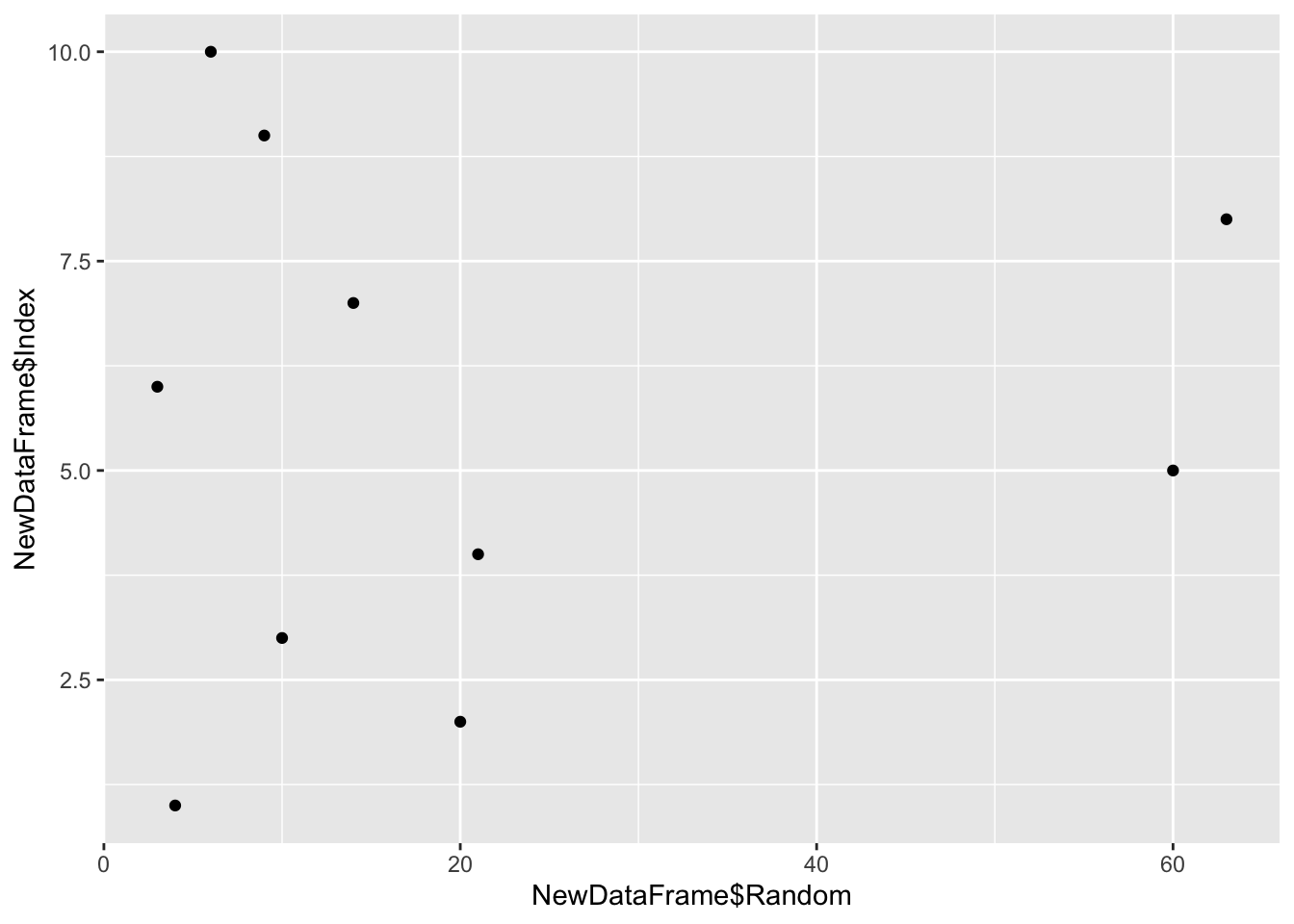
qplot(x = Random, y = Index, data = NewDataFrame)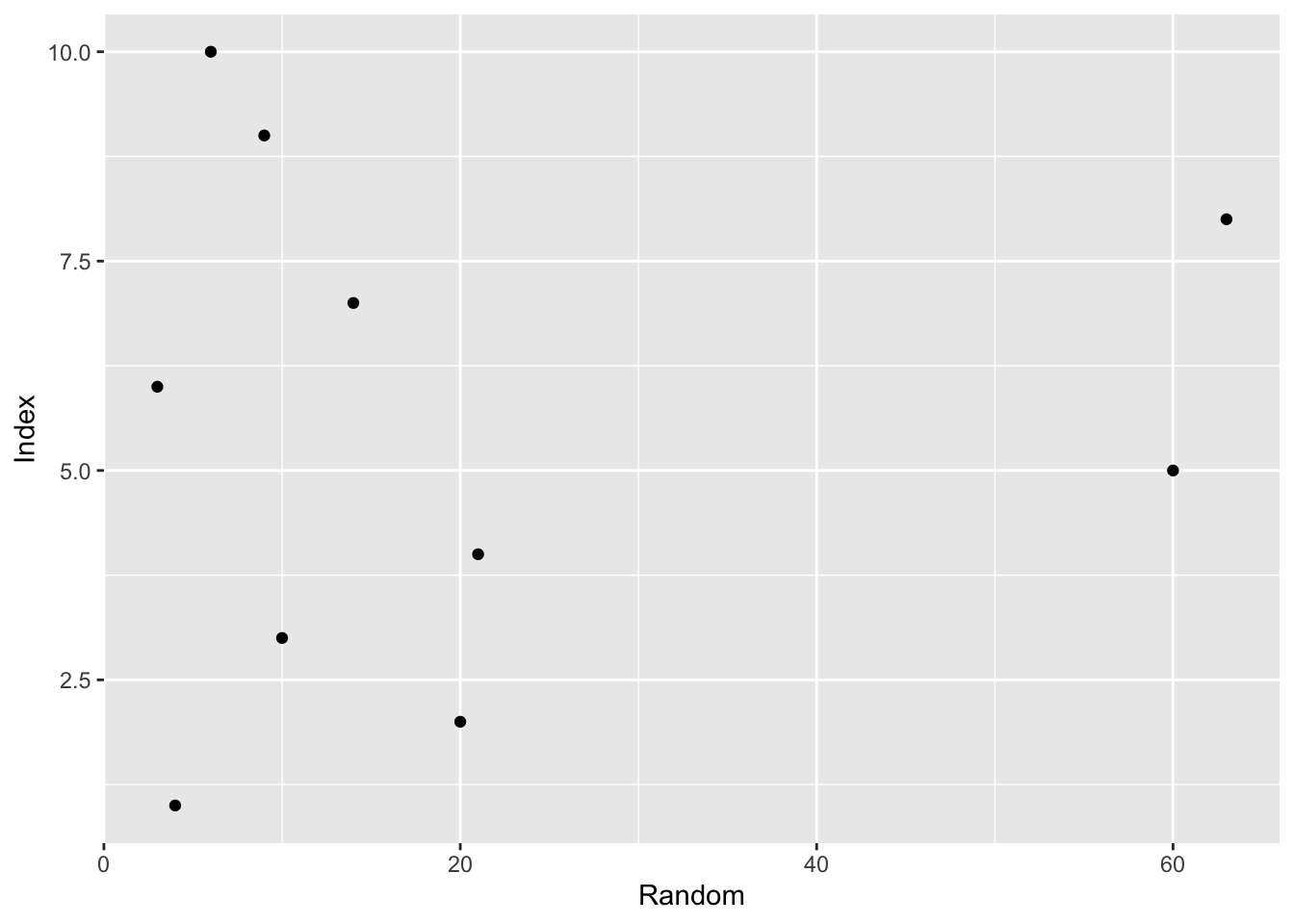
# We can change the size of our points by adding in the 'size' argument
qplot(x = NewDataFrame$Random, y = NewDataFrame$Index, size = 1)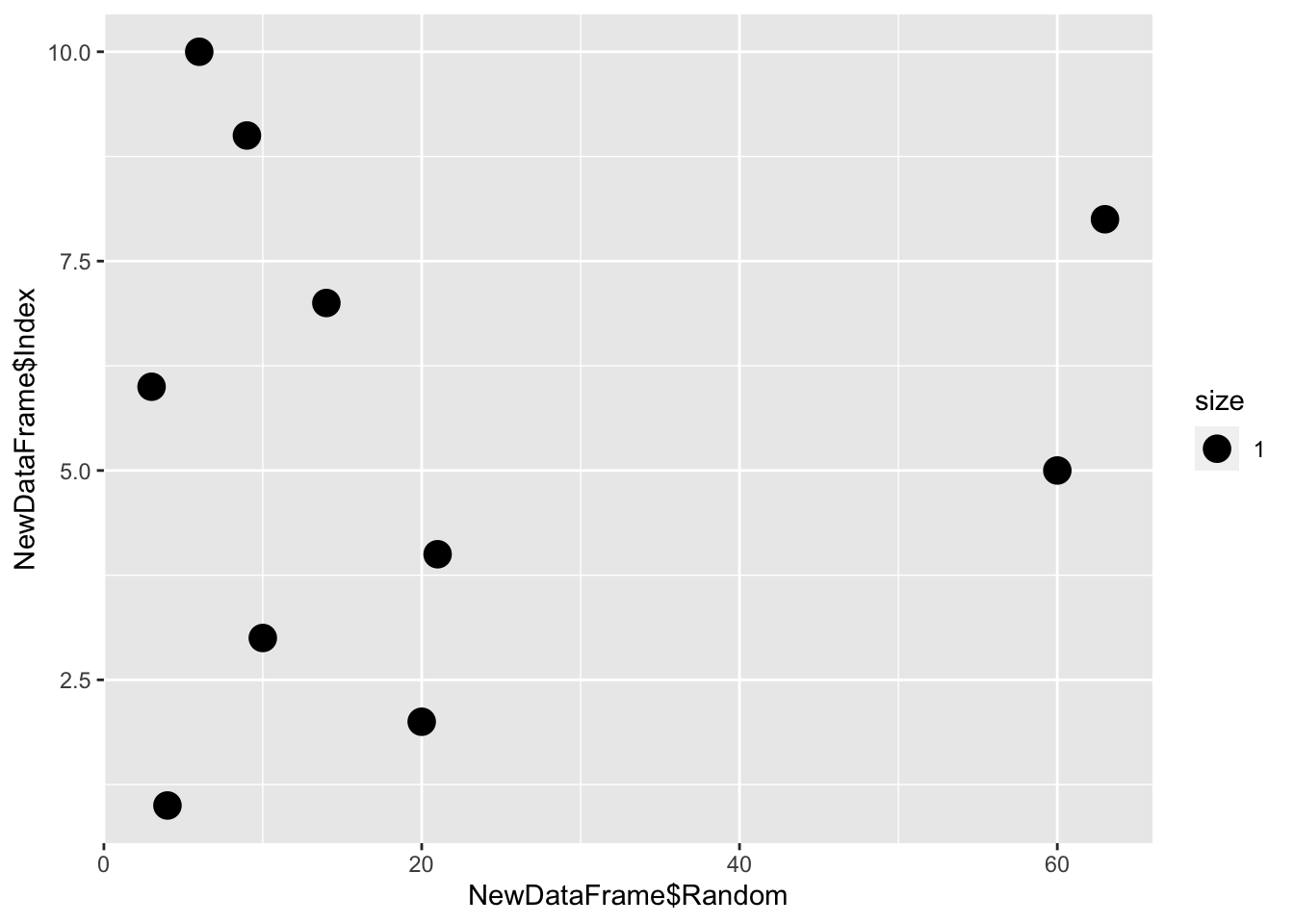
# Finally, we can add in coloring by a boolean logical
qplot(x = NewDataFrame$Random, y = NewDataFrame$Index, color = NewDataFrame$Index > 5, size = 1)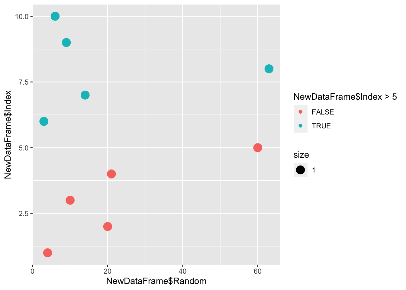
qplot(x = NewDataFrame$Random, y = NewDataFrame$Index, color = NewDataFrame$NewColumn, size = 1)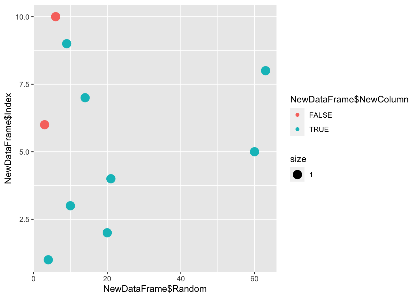
Exploring R
One of the most important things to do in R is read the documentation for different packages and functions. If we look at the function for qplot, it will give us the options for our plots.
We can do this by either running help(
help(qplot)
?qplot
This has lots of options, but the examples show where they have options for size and color. We’ll get into how to use these (and more!) in ggplot later, but you can explore how to visualize your own data using qplot, as long as you remember to load ggplot2 into your workspace.
You’ll notice that there’s an option for geom. This is the type of plot that will be made, and the default is a scatter plot (so geom = “point”). You can find this in the defaults for geom.
#Make a scatter plot
qplot(x = Index, y = Random, data = NewDataFrame,
      geom = "point",
      xlim = c(0,25), ylim = c(0,100),
      main = "Title of Randomness",
      xlab = "Index Expanded",
      ylab = "Random Numbers",
      color = Random > 5, size = 1)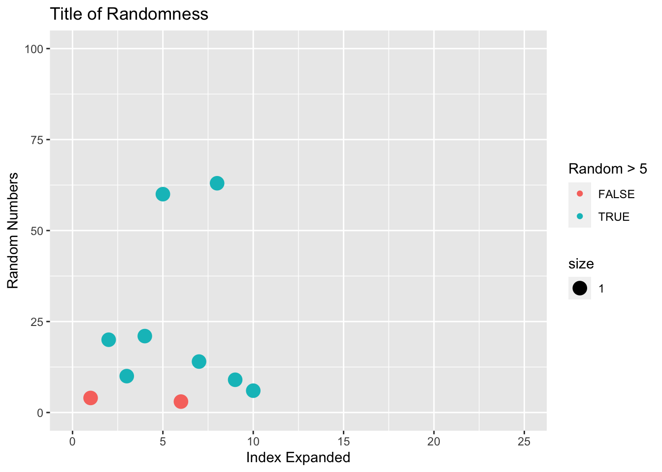
#Make a box plot with scatter (called jitter)
qplot(x = Random, y = NewColumn, data = NewDataFrame,
      geom = c("boxplot", "jitter"),
      main = "Boxplot of Random Numbers",
      color = Index)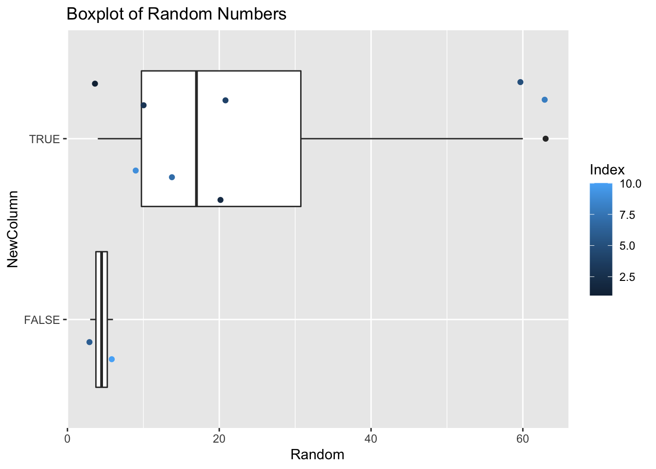
Practice
Load in the dataset penguins.csv, and plot the bill length vs body mass of penguins, coloring by species and changing the shape by island.
#Load in the csv using read.csv()

#View the data by using head() and find the names of the columns using str()

#Use qplot to plot the columns that you're interested in
Advanced Practice
Using either dplyr or subsetting, plot the Gentoo penguins bill length vs body mass, and color by if their body mass is above 5500.
# Your code below