Hands-On Data Wrangling

Last updated on 2022-06-21 Handout

Loading data

Following what we did last week, we are going to keep working with the penguins today. You can find the dataset after you extracted session3.zip which you can download from here.

Figure things out on the internet

If you don’t remember how to do something with R and happen to be the most R-fluent people in the peer, don’t panic. Most of the time, searching for [what you want to do] in R work out great.

Online forums like StackOverflow and Kaggle often give great answers with code examples that you could play with. If you are a genomic person, Biostar and SEQanswers would be your friend.

library(dplyr)

## 
## Attaching package: 'dplyr'

## The following objects are masked from 'package:stats':
## 
##     filter, lag

## The following objects are masked from 'package:base':
## 
##     intersect, setdiff, setequal, union

# How do you load a csv file with R?
penguins <- read.csv("penguins.csv")

Figuring things out within R

Oftentimes, an answer you found online provides a code that almost works, but you might not yet know enough to make it work. For times like this, R has documentation built in for each function describing the arguments that you can tweak and what it meant.

You can trigger the help page with ?[function] in the console. Let’s try it out: We used head() last week to take a glimpse of the first few rows of a table, so how do we print the first 3 instead of 6 rows?

head(penguins, n = 3)

##   species    island bill_length_mm bill_depth_mm flipper_length_mm body_mass_g
## 1  Adelie Torgersen           39.1          18.7               181        3750
## 2  Adelie Torgersen           39.5          17.4               186        3800
## 3  Adelie Torgersen           40.3          18.0               195        3250
##      sex year
## 1   male 2007
## 2 female 2007
## 3 female 2007

`count()` things

How many penguins of each species were observed on each island?

penguins %>%
  count(island, species)

##      island   species   n
## 1    Biscoe    Adelie  44
## 2    Biscoe    Gentoo 124
## 3     Dream    Adelie  56
## 4     Dream Chinstrap  68
## 5 Torgersen    Adelie  52

Which species is found on all islands? I know it’s obvious, but let’s use a sledgehammer to crack a nut this time.

# The output in the previous chunk is also a table that could be count()ed.
penguins %>%
  count(island, species) %>%
  count(species)

##     species n
## 1    Adelie 3
## 2 Chinstrap 1
## 3    Gentoo 1

`filter()` out your species

Let’s say you are interested in comparing how the islands influences the growth of penguins. Either you’ll need to go to Antarctica to observe more Gentoo or Chinstrap penguins on other islands, or only Adelie penguins make sense for your purpose.

# Since none of us is going to leave for Antarctica any time soon (right?)
# Let's keep only the Adelie penguins, and **assign it to a new object**.
adelie <- penguins %>%
  filter(species == "Adelie")

Revisiting the criteria for `filter()`

There are 6 basic types of comparison:

==: Equal to
!=: Not equal to
>: Larger than
>=: Larger or equal to
<: Less than
<=: Less than or equal to

# How many male Adelie penguins were observed?
adelie %>%
  filter(sex == "male") %>%
  count()

##    n
## 1 73

# How many Adelie penguins were found on islands that are not Dream island?
adelie %>%
  filter(island != "Dream") %>%
  count()

##    n
## 1 96

# How many Adelie penguins were observed during or before 2008?
adelie %>%
  filter(year <= 2008) %>%
  count()

##     n
## 1 100

Combining criteria

Sometimes, we’ll need more than one criteria to get the data we want. For example, if you are interested in the female Adelie penguins on the Biscoe island:

adelie %>%
  filter(sex == "female", island == "Biscoe")

##    species island bill_length_mm bill_depth_mm flipper_length_mm body_mass_g
## 1   Adelie Biscoe           37.8          18.3               174        3400
## 2   Adelie Biscoe           35.9          19.2               189        3800
## 3   Adelie Biscoe           35.3          18.9               187        3800
## 4   Adelie Biscoe           40.5          17.9               187        3200
## 5   Adelie Biscoe           37.9          18.6               172        3150
## 6   Adelie Biscoe           39.6          17.7               186        3500
## 7   Adelie Biscoe           35.0          17.9               190        3450
## 8   Adelie Biscoe           34.5          18.1               187        2900
## 9   Adelie Biscoe           39.0          17.5               186        3550
## 10  Adelie Biscoe           36.5          16.6               181        2850
## 11  Adelie Biscoe           35.7          16.9               185        3150
## 12  Adelie Biscoe           37.6          17.0               185        3600
## 13  Adelie Biscoe           36.4          17.1               184        2850
## 14  Adelie Biscoe           35.5          16.2               195        3350
## 15  Adelie Biscoe           35.0          17.9               192        3725
## 16  Adelie Biscoe           37.7          16.0               183        3075
## 17  Adelie Biscoe           37.9          18.6               193        2925
## 18  Adelie Biscoe           38.6          17.2               199        3750
## 19  Adelie Biscoe           38.1          17.0               181        3175
## 20  Adelie Biscoe           38.1          16.5               198        3825
## 21  Adelie Biscoe           39.7          17.7               193        3200
## 22  Adelie Biscoe           39.6          20.7               191        3900
##       sex year
## 1  female 2007
## 2  female 2007
## 3  female 2007
## 4  female 2007
## 5  female 2007
## 6  female 2008
## 7  female 2008
## 8  female 2008
## 9  female 2008
## 10 female 2008
## 11 female 2008
## 12 female 2008
## 13 female 2008
## 14 female 2008
## 15 female 2009
## 16 female 2009
## 17 female 2009
## 18 female 2009
## 19 female 2009
## 20 female 2009
## 21 female 2009
## 22 female 2009

What if you need penguins with extreme body weight? Say either over 4700g or below 2900g.

adelie %>%
  filter(body_mass_g > 4700 | body_mass_g < 2900)

##   species island bill_length_mm bill_depth_mm flipper_length_mm body_mass_g
## 1  Adelie Biscoe           36.5          16.6               181        2850
## 2  Adelie Biscoe           36.4          17.1               184        2850
## 3  Adelie Biscoe           41.0          20.0               203        4725
## 4  Adelie Biscoe           43.2          19.0               197        4775
##      sex year
## 1 female 2008
## 2 female 2008
## 3   male 2009
## 4   male 2009

Logical operations: What’s happening under the `dplyr` table

Essentially, what filter() relies on is to ask a series of yes/no question to each row of a column, and the answers to these yes/no questions are called Boolean or logical values.

In R, TRUE means yes, while FALSE means no.

# Is 3 larger than 5?
3 > 5

## [1] FALSE

# Is 2022 equal to 2020?
2022 == 2020

## [1] FALSE

# Is "apple" not equal to "orange"?
"apple" != "orange"

## [1] TRUE

These logical values can be further calculated with & (AND), | (OR), and xor().

	`&`	`\|`	`xor()`
TRUE/TRUE	TRUE	TRUE	FALSE
TRUE/FALSE	FALSE	TRUE	TRUE
FALSE/TRUE	FALSE	TRUE	TRUE
FALSE/FALSE	FALSE	FALSE	FALSE

So, how many Adelie penguins either have a bill length shorter than 35mm or a bill depth below 15mm?

adelie %>%
  filter(bill_length_mm < 35 | bill_depth_mm < 15) %>%
  count()

##   n
## 1 9

Now that we know filter() is working with logical values, you won’t be surprised that it can also use other functions that gives a logical value as its output as a criterion.

For example, we mentioned that NA is how R labels missing data. Since we are interested in body weight, we might want throw away rows with missing body weight…

# You might want to try filtering for body_mass_g== NA
adelie %>%
  filter(body_mass_g == NA)

## [1] species           island            bill_length_mm    bill_depth_mm    
## [5] flipper_length_mm body_mass_g       sex               year             
## <0 rows> (or 0-length row.names)

What is happening? Remember that we said R treats NA very differently. As a matter of fact, almost every operation gives you NA when NA is involved.

# Try these
5 == NA

## [1] NA

3 > NA

## [1] NA

"North America" != NA

## [1] NA

3.1415926 <= NA

## [1] NA

Since NA is missing data, this actually makes sense:

5 == NA is like asking “is 5 equal to something I don’t know?”, and the answer has to be “I don’t know”.

So, how do we ask R if it doesn’t know something or has an NA there? We use is.na().

is.na(NA)

## [1] TRUE

is.na("National Academy")

## [1] FALSE

You can use is.na() with filter() to find the rows where body weight is NA.

# Use is.na() to get rows with NA in body_mass_g
adelie %>%
  filter(is.na(body_mass_g))

##   species    island bill_length_mm bill_depth_mm flipper_length_mm body_mass_g
## 1  Adelie Torgersen             NA            NA                NA          NA
##    sex year
## 1 <NA> 2007

How do we select all other rows then? In R, ! flips a logical value, and you can pronounce it as not.

# Not TRUE
!TRUE

## [1] FALSE

# Not FALSE
!FALSE

## [1] TRUE

# Flipping (3 > 5)
!(3 > 5)

## [1] TRUE

We can use ! to find rows that are not NA.

# How many Adelie penguins have their body mass recorded?
adelie %>%
  filter(!is.na(body_mass_g)) %>%
  count()

##     n
## 1 151

Extended reading: Dealing with missing values

Depends on what you work with, you might not always want to drop missing values.

If you are not going to throw those data away, you’ll need to ask yourself questions like “Does missing value appear randomly?”, and decide how to best deal with them.

If you are interested, Hadley Wickham has a section in his book R for Data Science discussing this.

Group your data for further analysis

Let’s say we are interested in how body weight differs between islands. To perform this analysis, we might want to calculate the median and standard deviation of body mass per island.

To indicate how dplyr should group your data, we use group_by() to tell it which column contains the group labels.

Let’s assign the grouped data to another object named adelie_per_island

adelie_per_island <- adelie %>%
  filter(!is.na(body_mass_g)) %>%
  group_by(island)

Get summary statistics with `summarize()`

Now that we grouped the data, we can calculate the summary statistics.

The syntax for summarize() is as follows:

# You tell summarize() which functions to use on which column
adelie_per_island %>%
  summarize(mean(body_mass_g))

## # A tibble: 3 × 2
##   island    `mean(body_mass_g)`
##   <chr>                   <dbl>
## 1 Biscoe                  3710.
## 2 Dream                   3688.
## 3 Torgersen               3706.

By default, the column names of the summary table is the function call we gives to summarize(), which could be a bit ugly. We can rename the columns by:

adelie_per_island %>%
  summarize(mean_bw = mean(body_mass_g))

## # A tibble: 3 × 2
##   island    mean_bw
##   <chr>       <dbl>
## 1 Biscoe      3710.
## 2 Dream       3688.
## 3 Torgersen   3706.

The summary statistics that we use the most often are:

Arithmetic mean (mean())
Median (median())
Standard deviation (sd())

Let’s summarize the data with median and standard deviation per island.

# Summarize the Adelie subset per island with the median and standard deviation 
# of the body mass
adelie_per_island %>%
  summarize(bw_median = median(body_mass_g), bw_sd = sd(body_mass_g))

## # A tibble: 3 × 3
##   island    bw_median bw_sd
##   <chr>         <dbl> <dbl>
## 1 Biscoe         3750  488.
## 2 Dream          3575  455.
## 3 Torgersen      3700  445.

What if you don’t group?

adelie %>%
  filter(!is.na(body_mass_g)) %>%
  summarize(bw_median = median(body_mass_g), bw_sd = sd(body_mass_g))

##   bw_median    bw_sd
## 1      3700 458.5661

What if you want to group with another grouping variable?

# Let's group with sex
adelie %>%
  filter(!is.na(body_mass_g), !is.na(sex)) %>%
  group_by(sex) %>%
  summarize(bw_median = median(body_mass_g), bw_sd = sd(body_mass_g))

## # A tibble: 2 × 3
##   sex    bw_median bw_sd
##   <chr>      <int> <dbl>
## 1 female      3400  269.
## 2 male        4000  347.

A picture is worth a thousand words

While it’s great to have summary statistics, oftentimes a quick visualization of our data will be very helpful.

qplot() provided by ggplot2 is designed for this purpose and can be easily incorporated into your pipeline.

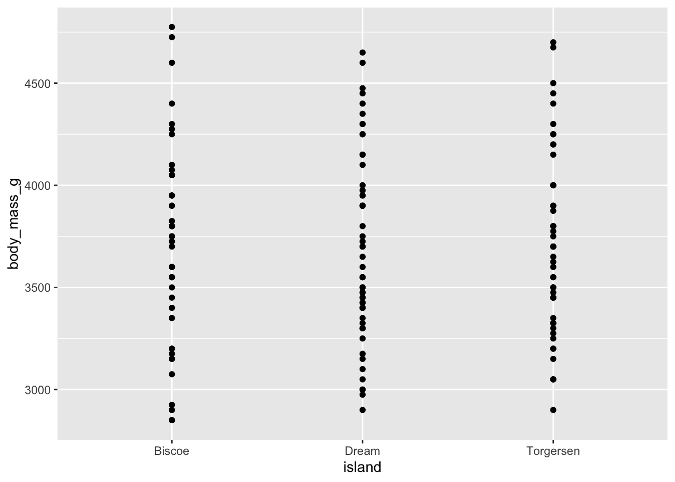
Example: a quick scatter/strip plot per island

Let’s plot something with points on a plane where the x-axis is the islands and the y-axis is the body weight.

# Load ggplot2
library(ggplot2)

adelie_per_island %>%
  qplot(data = ., x = island, y = body_mass_g, geom = "point")

There several required arguments for qplot():

data: The data you want to plot.
x: The column name of the variable you want to use as the x-axis
y: The column name of the variable you want to use as the y-axis
color: The column name of the variable you want to color your plot by
geom: Short for “geometry”, the type of plots you want to do. Popular ones include:
- point
- bar
- boxplot
- violin
- histogram
- density

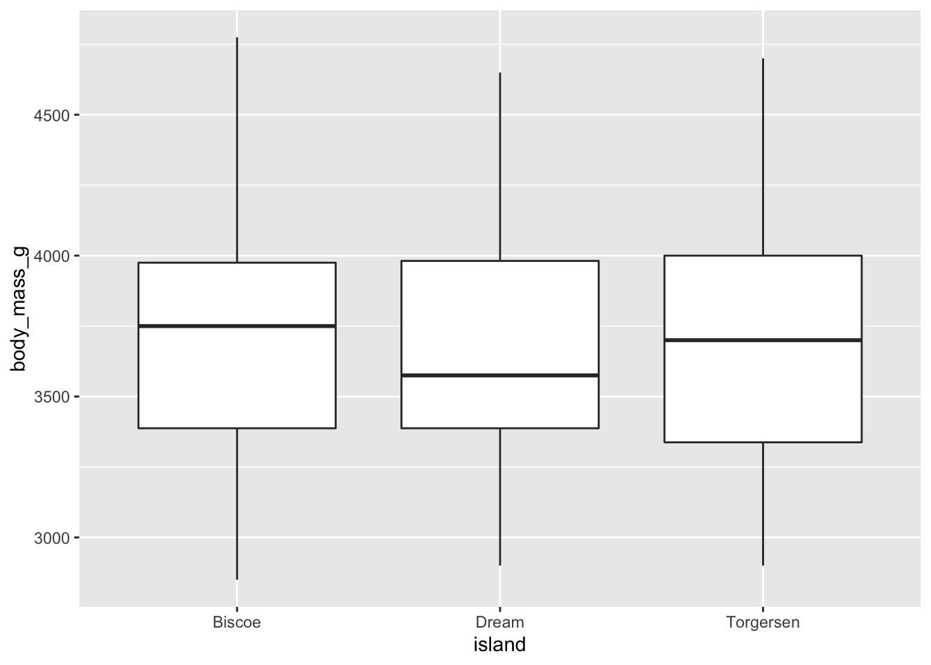
# Let's do a boxplot instead
adelie_per_island %>%
  qplot(data = ., x = island, y = body_mass_g, geom = "boxplot")

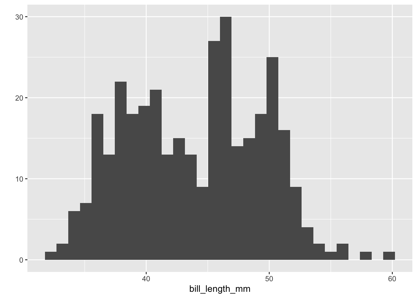
### What is the distribution of bill lengths of the whole dataset?

# Plot a histogram with bill lengths on the x-axis
penguins %>%
  qplot(data = ., x = bill_length_mm, geom = "histogram")

## `stat_bin()` using `bins = 30`. Pick better value with `binwidth`.

## Warning: Removed 2 rows containing non-finite values (stat_bin).

Is bill length and depth correlated for the Adelie penguins?

# Plot a point plot with bill length on the x, bill depth on the y, and
# color by sex
adelie %>%
  qplot(
    data = .,
    x = bill_length_mm,
    y = bill_depth_mm,
    color = sex,
    geom = "point"
  )

## Warning: Removed 1 rows containing missing values (geom_point).

Yen-Chung Chen

PhD Candidate

A graduate student interested in developmental biology, neurobiology and bioinformatics.