Prepare your computer for R
AGENDA
- Introductions
- Installing R
- This Worksheet :)
Adpated from material curated by Eugene Plavskin and Grace Avecilla
Exploring RStudio
- The console: Where you run commands one by one (bottom)
- The environment: Where you can see what is loaded in R (upper right)
- The file explorer: An easier way for you to find files (otherwise you’ll need to know the path of a file to use it in R; lower right)
Installing packages
Packages are like kits in experiments: They package the reagents and instructions for otherwise complicated processes for you.
We’ll be installing 3 packages today
# This is how we ask R to install packages
# R will try to ask several central repositories if they have this package
install.packages("rmarkdown")
Using Rmarkdown
Rmarkdown file allow you to record your thinking process (as text) along with your analyses (as code chunks).
Having why you are doing the analysis and the specific code for it will help you catch up faster if you ever need to go back to the same analysis again.
Text and code
This is a line of text:
“I know how to use R!”
# This is a chunk of code. Do you notice that the background looks different?
# Also there is three buttons at the upper right corner

# Press the _play_ button, and the output will be shown below the chunk
print("I know how to use R")
## [1] "I know how to use R"2+2## [1] 4Running code:
Click on the run button on the upper-right corner of a chunk
Ctrl + Enter (Windows) / Cmd + Return (Mac)
Generating output
- Click the knit button on the upper rim of the editor
- Knitting will re-run all your code in the file from scratch, which is a
good thing because it makes sure:
- The code works on its own
- We haven’t accidentally deleted or added some lines of code that will break the code.
Working directory and Rstudio projects
What is a working directory?
A working directory is where R will try to find things if you ask it to1.
Checking and setting your working directory
You can check the path of your working directory with getwd()
(short for get working directory).
# Expect to see a path printed below
# This is where R find things for you
getwd()
## [1] "/Users/ycc/Dropbox/Docs/NYU/Teaching/SURP/NYU_SURP_blogdown/content/handout/2022-06-13-prepare-your-computer-for-r"Loading files from your working directory
Now that you have a directory, files inside that directory can be loaded using
functions like read.csv(). This function will take a comma-separated file
(which you can make in Excel) and allow you to save it as a variable that R can
work with.
For the example below, mytestdata.csv can be found in the example data.
# Open the csv file with Excel or Google Sheet to take a look
# mytestdata

# And then we load it to see how it looks like in R
read.csv("mytestdata.csv")
## Day Count Group
## 1 1 12 1
## 2 1 15 2
## 3 2 8 1
## 4 2 3 2
## 5 3 10 1
## 6 3 24 2# You need to ask R to keep the csv files
# *Check the environment tab on the upper right corner of your window
mytestdata <- read.csv("mytestdata.csv")
# You can ask R to retrieve what it keeps later by the name you gave to the data
mytestdata## Day Count Group
## 1 1 12 1
## 2 1 15 2
## 3 2 8 1
## 4 2 3 2
## 5 3 10 1
## 6 3 24 2Basic usage of R: Using it as a calculator
Enter the following line of command in the console
17 + 2.3## [1] 19.3In programming, division is often written as slashes (/), while
multiplication is written as asterisks (*). Now, let’s try doing these in the
console as well:
# Try multiplying 8 by 7

8*7
## [1] 56# Try dividing 48 by 12
48/12## [1] 4An example of our data
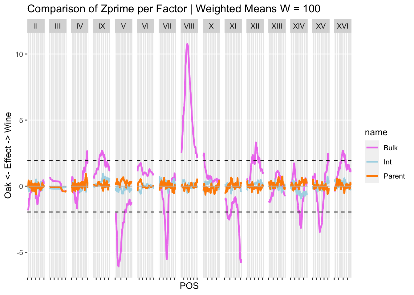
Cassandra’s data is allele frequencies as read counts from sequencing. To analyze it, she first:
- loads in the data,
- runs an R function to analyze it,
- plots using
ggplot2.
Here is a quick version of this:
library(ggplot2)
library(dplyr)
##
## Attaching package: 'dplyr'## The following objects are masked from 'package:stats':
##
## filter, lag## The following objects are masked from 'package:base':
##
## intersect, setdiff, setequal, unionlibrary(tidyr)
#Read in the data
WeightedMeanZStats.100 <- read.csv("CBData.csv")
#Look at the data (this only prints the first 6 rows)
head(WeightedMeanZStats.100)## X CHROM POS Bulk Parent Int Stat
## 1 result.1 II 100153 -2.3893709 -1.0534663 1.64175559 Z
## 2 result.2 II 100367 -0.9361101 -0.2837268 0.55031705 Z
## 3 result.3 II 100413 -1.1028976 -0.6802854 0.95854049 Z
## 4 result.4 II 100878 0.7191787 0.9999416 -1.25245792 Z
## 5 result.5 II 101289 -1.2163032 1.4995884 0.07063202 Z
## 6 result.6 II 101340 -1.4019217 1.1382948 -0.29809070 Z#Find the dimensions of the datast
dim(WeightedMeanZStats.100)## [1] 95106 7unique(WeightedMeanZStats.100$Stat)## [1] "Z" "ZPrime"#Plot the data using ggplot (which we'll go into more later!)
WeightedMeanZStats.100 %>% filter(Stat == "ZPrime") %>% pivot_longer(c("Bulk", "Parent", "Int")) %>%
ggplot(., aes(x = POS, y = value, color = name)) + geom_line(size = 1) + #geom_point(alpha = 0.1) + #+
geom_hline(yintercept = 0, color = "gray") +
geom_hline(yintercept = c(1.96, -1.96), color = "black", linetype = "dashed") +
theme(axis.text.x = element_blank()) + ylab("Oak <- Effect -> Wine") +
scale_color_manual(values = c("violet", "lightblue", "darkorange")) +
facet_grid(~CHROM, scales = "free") + ggtitle("Comparison of Zprime per Factor | Weighted Means W = 100")
See working directory if you are interested.↩︎